INFINIWORKFLOW is a node-based platform for building AI, ML, and Computer Vision pipelines, with real-time support for sensor acquisition and device control.
Rapid Prototyping (No Coding)
Intuitive Browser-Based UI
GPU Accelerated (Performance)
Comprehensive toolset (over 900+ tools)
Enhanced with integrated AI tools
Automatic Code Generation for integrating to your app
User Interface Elements
INFINIWORKFLOW runs entirely in your browser. Its main UI components are:
The HUB portal provides a comprehensive overview of the system's capabilities, hardware compatibility, and the latest software advancements. To open the information overlay, click the HUB icon located in the toolbox. The following functions are available at the HUB:
Showcase: View high-level video demonstrations and a detailed "What's New" timeline tracking monthly software improvements.
Summary: Access a general overview of the platform, highlighting core features such as rapid no-code prototyping and the browser-based UI.
Benefits: Review the specific advantages of the architecture, including its modular node-based logic and system scalability.
Platforms: Check hardware and OS compatibility, ranging from standard desktop environments (Windows, OSX, Linux) to edge computing hardware like NVIDIA Jetson.
Markets: View details regarding localized support for international regions, specifically English, Japanese, and Chinese users.
Packages: View latest packages that you can extend the capabilities - see Downloadable Packages.
What's New: See the latest tools and user-interface features.
App Menu
The App Menu is a floating toolbar docked to the top of the canvas, providing the following functionality:
Example: the real App Menu toolbar (a floating bar docked to the top of the canvas - hover peeks it, pin it open with the pin icon on the left)
||
Hover any icon above to see its name - the same tooltip behavior as the real toolbar. Gold icons open AI features, red icons are destructive (New Workflow/Exit), and the underlined icons on the left each expand into their own popout menu (File, Edit, Workflow Graph, Customize, Windows, Performance, Artificial Intelligence, Studios, Settings, Help) - listed in full below.
Hide and Show the Toolbox
File
Load Workflow: opens an existing workflow from the demos folder using the Browser
Save Workflow: saves the workflow using the Browser. First it shows what changed since the file was last saved, diff style: nodes added (green +), removed (red −) and edited (amber ~, each parameter shown as old → new, and multi-line values such as notes and code as a line-by-line diff), edges added and removed, nodes moved, and group, bookmark, publish and resolution changes. A summary row counts each kind of change, and a mini map on the right shows the graph with added nodes green, edited amber, removed ones as red dashed ghosts where they used to be and moves as blue arrows. Hover a change to find it on the map, or click it to select that node on the canvas. Press Enter or Proceed... to go on to the Browser, where the file is saved, Esc to cancel. Untick Show changes before saving to go straight to the Browser from then on; Shift+click Save Workflow still shows the changes. A workflow that has never been saved goes straight to the Browser.
Rate & Label Workflow: opens the Workflow Info panel for the workflow's author, description, star rating, training label and requirements. It floats over the flowgraph like the Radar and does not block it: drag it by its header, resize it from the corner, and it reopens where you left it. Changes save as you type ("Saved" flashes in the header) and are written to the file with the workflow. It also opens from the button in the Radar's header, and follows along when you open another workflow.
Import Package: installs a package zip - a workflow with its extensions and assets - see Import & Export Packages
Export Package: zips the workflow with its extensions and every file it references into your Downloads folder - see Import & Export Packages
Clear: resets the workflow to start a new one from scratch
Exit the application
Edit
Undo will undo the last action
Redo will redo the prior action
Copy: copies the selected nodes and connected edges to the clipboard
Paste: pastes a copy of the selected nodes and connected edges from the clipboard to the workflow. The copied nodes will all be renamed to have unique names in the workflow
Cut: deletes the selected nodes and connected edges and pastes them to the clipboard
Duplicate: duplicates the selected nodes and connected edges to the workflow. The duplicated nodes will all be renamed to have unique names in the workflow
Delete: deletes the selected nodes and connected edges
Workflow Graph
Zoom out the flowgraph so you can see more of the nodes in the workflow
Zoom fit the flowgraph to show the default zoom and pan which will show all the nodes in the workflow
Zoom in the flowgraph so you can see focus on the nodes in center of the workflow
Find a node in the flowgraph, adjusts the viewport and selects the node
Auto arrange the nodes: lays the graph out left to right in columns, following the edges, ordering each column to
reduce crossing edges and spacing nodes by their real size. Separate, unconnected parts of the graph are stacked one above the other.
With two or more nodes selected only those are arranged, and they stay where they were on the canvas; with zero or one selected the
whole graph is arranged. Either way the view then zooms to fit what was arranged. Sticky notes are never moved. Auto arrange can be undone and redone
Select/deselect before: allows you to change selection of the nodes before the current node in your flowgraph
Select/deselect after: allows you to change selection of the nodes after the current node in your flowgraph
Radar: an overview window of the whole flowgraph. It is set from the Radar button at the top of the App Menu toolbar (no longer in this menu): automatic (the default - it appears only when nodes are off screen), always shown or off. The Radar window can be dragged by its title bar and resized from its corner, and remembers where you left it. Its pin keeps it showing even when every node is on screen; unpin to go back to automatic, fit zooms the graph so every node is on screen, or to turn it off. Inside the window, drag the blue rectangle to pan, click anywhere to jump there, and scroll to zoom. Grey boxes are nodes, blue is the selection and green is the node in the Viewer. The Radar button among the always-shown buttons at the top of the App Menu toolbar opens a small menu to pick Always shown, Automatic (only when nodes are off screen) or Off, with the current choice ticked. The button itself shows the mode: blue while always shown, dimmed while off. Pinning or closing the Radar from its own window updates the button, and the menu's tick if it is open.
The row of numbers along the bottom holds the four viewport bookmarks:
click an empty number to bookmark the current view, click a yellow one to jump to it, Shift+click to overwrite it and right click to
clear it. Bookmarked views are drawn on the radar as yellow dashed rectangles
Lenses: extra views of the flowgraph, each with its own zoom and pan, opened from the buttons at the right of the Radar's bottom row. Split View ×2 and ×4 tile lenses over the flowgraph; pane 1 to 4 opens viewport bookmark 1 to 4 when that bookmark is set, fitting the whole bookmarked area into the pane; panes without a bookmark start out showing exactly what was under them, so an unbookmarked split looks unchanged until you pan (drag empty space) or zoom (scroll) one of them. Floating Lens opens one movable, resizable window. In a lens you can select nodes (Shift adds to the selection), drag them (undo works as usual) and double-click one to View & Edit it; connecting edges and the right-click menus stay in the main view. Press F with the mouse over a lens to fit all nodes in that lens. Hover a lens for its header: the 1–4 chips work like the Radar's - click an empty one to bookmark what the lens shows, a filled one to take the lens there, Shift+click to overwrite - and the one the lens is showing is lit; shows that lens's view in the main flowgraph and closes the lenses, fits all nodes in the lens, closes all the lenses and returns to the normal view. Close Lenses (shown in the Radar while lenses are open) closes them all. Lenses are live: thumbnails, Python displays (tables, charts), profiling colours and edits made anywhere show up in every lens. While lenses are open the menu toolbar auto-hides (hover the top edge to bring it up) and goes back to its pinned state when the lenses close. Opening a node with View & Edit hides the lenses and pins the menu toolbar again; clearing View & Edit brings the lenses back as they were and auto-hides the toolbar again. The Radar outlines each open lens's area in that lens's colour (L1, L2...), beside the dashed bookmark rectangles.
Customize
Rename: allows you to modify the name of the node. The name is initially set to be based on the Tool's name but
will automatically be made a unique name by prefixing with numbers.
You can also rename without the menu: click a node's title once and it becomes editable in
place, with the whole name selected so typing replaces it - Enter or clicking away keeps the
new name, Escape abandons it. Dragging a node by its title still works; only a click that
does not move starts editing. Zoomed far enough out that the name is no longer readable, clicking it
does nothing and this menu entry is the way to rename - the hint under the name disappears at the
same point, so it is clear which is which. Double-clicking a node remains View & Edit.
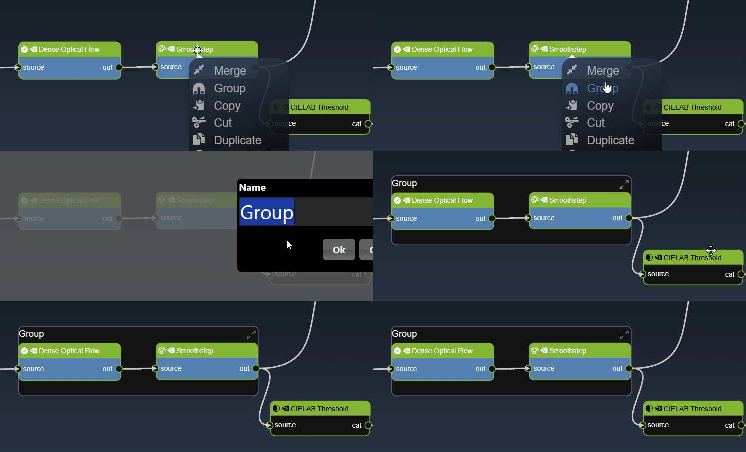
Group: for the selected nodes, allows you to group them together and become child nodes of the group. See Group Nodes
Ungroup: for the selected group node, allows you to ungroup to revert the child nodes. See Group Nodes
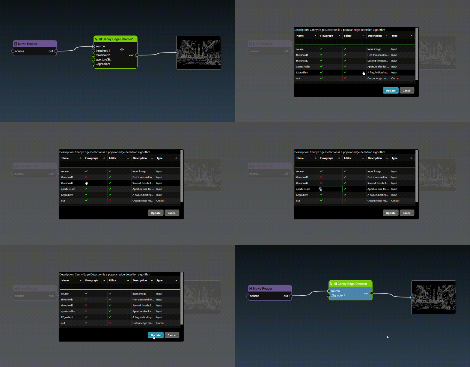
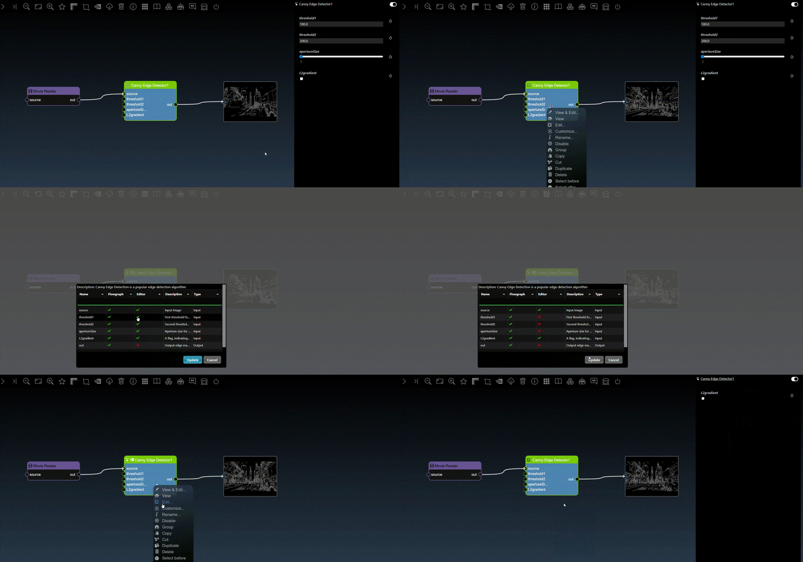
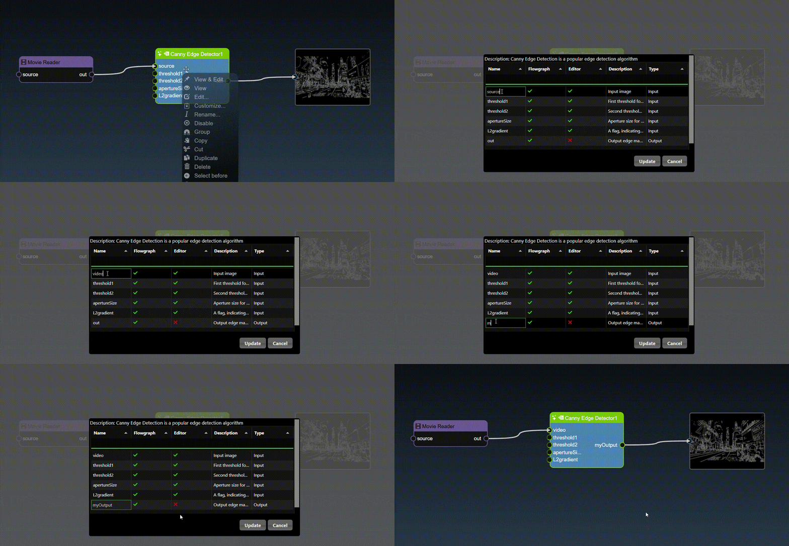
Customize: for the selected node, allows you to hide or show the inputs and outputs
in either the flowgraph or editor, as well as change the names of the inputs and outputs. See Customize Nodes
Export Group: for the selected group node, allows you to export it to a new tool. See Group Nodes
Insert/Remove Input and Output have moved onto the node itself (see Adding and Removing Ports): select a single node that allows dynamic inputs or outputs and small + / − buttons appear just below it - the left pair adds or removes an input, the right pair an output. − is greyed out when the last input is mandatory or connected, since only an unused last input can be removed
Save as Custom Node: for the selected node, creates a new reusable node with the node's current settings as its defaults, packaged with its asset files into a zip in your Downloads folder that you can share with others. To package a whole workflow use Export Package instead
Windows
HUB, Platform Information, Packages & What's New & More
Generate App Code: generates code for integration into your application - see Code Generator
Generative AI chatbox (Claude or ChatGPT) that can build/edit workflows, generate plugins, run AI Studio, and more from natural-language prompts
AI Studio allows you to label movies, fine-tune models and create segmentation inference tools
Live Tiles: swaps the flowgraph for a grid of live node outputs - the same switch as the button on the App Menu bar
Dashboards: live KPI tiles, charts, gauges, heat maps and camera views, with alerts and scheduled PDF reports
Documents: reports with live blocks that are frozen when signed
Analytics Studio: one flat list of every saved workflow that has dashboards, sheets, documents or an app; pick one and it opens straight into it
Solution Studio: the whole app (cameras, detectors, events, dashboards) as one spec stored with the workflow; Write with AI builds it from a description
Roadmap: the Analytics overview, the Ideas backlog and the feature Mockups, full screen
Displays the rendering status console which also indicates progress, warnings and errors
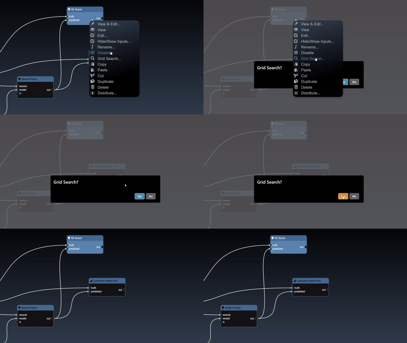
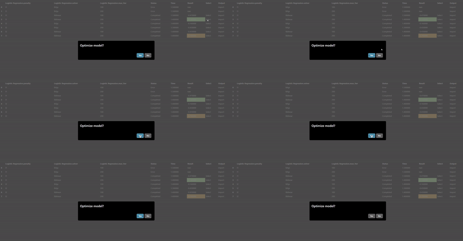
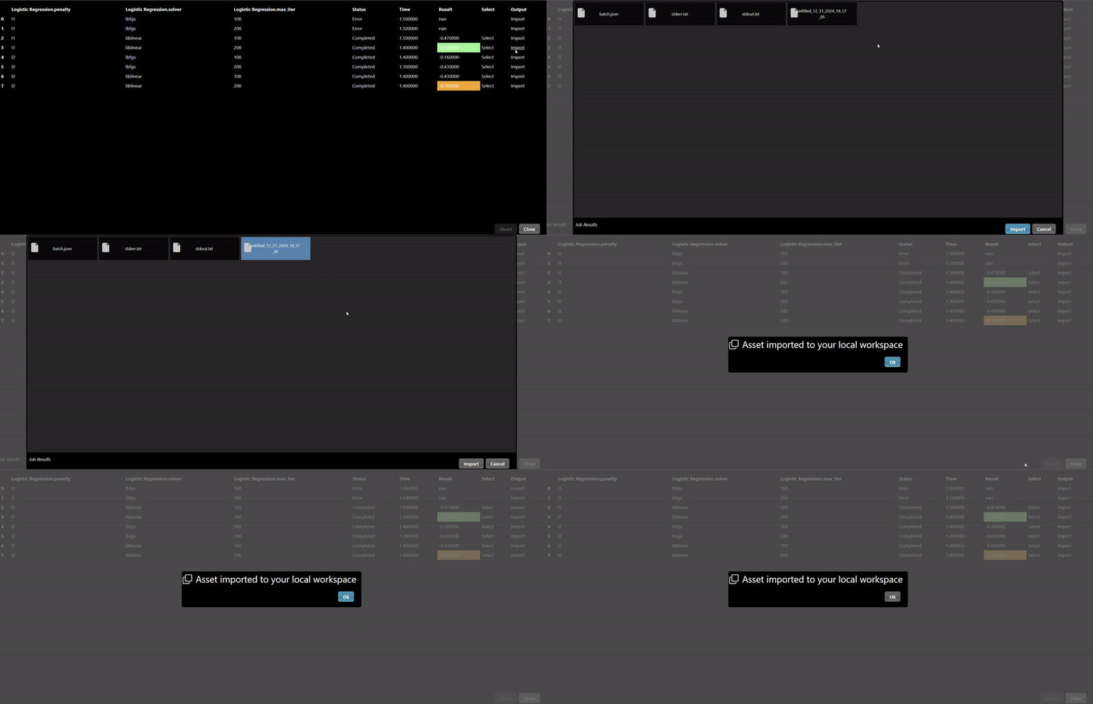
Shows the Grid Search dialog that is used to optimize your ML models using the GridSearch UI
Remote Script Execution: opens the Remote Script Execution dialog, a standalone way to run a Python script on this machine or a peer without touching your workflow's nodes.
Performance
Profile (P): shows a live FPS speed-dial badge on every active node and labels each edge with what flows through it - see Profile for details.
Network Manager: opens the Network Manager dialog, for running part of your workflow on a different process or a different machine on the network - the same dialog's Render mode instead captures one node's output(s) straight to disk; see Render to Clip for details.
Optimization Studio: measures the workflow's AI nodes with OpenCV FP32, FP16 and NVIDIA TensorRT on the workflow's own frames, checks the results match, and applies TensorRT where it is faster with the same result.
Synchronize...: available when the selected node has 2 or more connected inputs. Opens the Synchronize dialog to bring branches that have drifted out of sync back into alignment - see Synchronize for details.
Live Tutorials: opens the tutorials browser - pick a tutorial and it plays itself on the canvas, showing each click and gesture. Click the button again while one is playing to cancel it
Opens a guide for mouse and touch gestures
About box: an animated splash - the InfiniWorkflow bonsai grows from its pot, glows and sways, with light flowing up the trunk - showing the build date. Click anywhere or press Esc to close it
Pauses all the selected playable nodes which is useful if you are tracking and want to position the tracker marker
Toolbox
The Toolbox is where you add new tools to your flowgraph as nodes.
The first tab shows every tool; the remaining tabs each show a subset, such as tools related to Computer Vision or ML. Hover over a tab icon to see
a tooltip with its category name. Once you've selected a category tab, you can further narrow the list by typing keywords into the search field -
useful for quickly finding a specific tool to insert into your workflow.
Example: the Toolbox docked at the bottom of the canvas - category tabs, search, and a grid of draggable tool tiles
Canny Edge
Find Contours
Movie Reader
YOLO8 Classification
ONNX Runtime
Widget: Slider
Tool tile colors indicate language: purple = C++, blue = Python, green = CUDA, orange = OpenCL, pink = OpenGL, gray = Widget. The highlighted tile shows a hover/selected state.
Toolbox Gestures
Hovering over a tool shows a tooltip describing it. You can insert a tool into the workflow using any of the following gestures:
Drag and Drop
Insert a node with edge automatically: select the node you wish to connect it to, then double click the tool - a new node is inserted with a link added automatically.
Insert new tool in between by dropping a node from the catalog over an edge - the edge highlights to show it can accept the drop.
Insert an existing node by dragging it over an edge, which highlights to show it can be inserted in between.
Insert new tool after a port: drag a node from the catalog and drop it over a port to connect an edge from that port.
Replace with a new tool by dropping it over the title
Rename node: click the title and type
Show/Hide node inputs: double click any input port
Toolbox Layouts
Infiniworkflow has several hundred nodes available, which allows for many possibilities but also can be daunting for new users or can stand in the way of users who
are only looking to build a specific application (if you are building a Data Science workflow, you probably don't need to see the many Color Correction nodes that are
available). As such, Layouts have been added as a feature for controlling which categories and nodes show up in your Toolbox. They are straightforward to use,
but by no means necessary to learn about if you do not wish to change how your Toolbox appears, so you may skip this section and not lose any critical information.
Layout can be defined as a set of categories, and the respective nodes inside them, that will appear within the Tool Bar if the Layout is selected. You can switch
between Layouts. By default the Layout is "All", as that shows
all categories and all nodes inside those categories. However, this is but 1 of a handful of pre-made Layouts that are available. These pre-made Layouts include
"Computer Vision", "Data Science", and "Machine Learning"; as can be expected, when we switch to one of those Layouts, only the categories / nodes relevant to the
respective topic (Computer Vision, for example) will appear. The video shows how the toolbar changes when switching between Layouts.
In addition to the Layouts seen here, users can also choose to add their own custom Layouts. To add a Layout, go to Settings, which can be found in the bottom right
side by the Layouts button, and click on the "New Layouts" option within Settings. Enter in your Layout name, and save. If you click on the Layouts button now, you
will now see that your new Layout has been added to the list of other Layouts, as shown here.
To begin changing how the categories / nodes appear within your Layout's Toolbox, click on the Layouts button and then click on the Layout you wish to change.
Now that you're in, you may begin moving both categories and nodes as you like. The following operations are possible:
I. Moving single Nodes into the Trash: these nodes no longer show up in the category they were in previously
II. Moving an entire Category to the Trash: the category is no longer in view, and all its nodes go to the Trash
III. Moving single Nodes into different Categories: the node's symbol is unchanged, but it now belongs to the new category
IV. Moving an entire Category into another Category: only the target category appears in the Toolbox list, holding all nodes from both
If you are unhappy with your Layout and want to start over, simply go to the Settings button and click on the "Reset Layout" button. Alternatively, you may delete the
Layout all together by clicking on the "Delete Layout" button within Settings. NOTE: Make sure that you are IN the Layout that you want to reset / delete, or you may
end up resetting / deleting the wrong Layout! Do this by clicking on the desired Layout after clicking the Layouts button before making any changes.
Flowgraph
The flowgraph is where you construct your workflow, which comprises Nodes and Edges. Nodes represent functions that take input and generate outputs.
You create nodes by dragging tools into your workflow from the Toolbox. A node's inputs and outputs have 'ports', which are where edges connect.
An edge connects the output port of an upstream node to the input port of a downstream node. Any input port left unconnected
can instead be set to a specific value using the Parameter Editor. A node's color indicates its execution language:
Adding an edge connects the output of an upstream node to the input of a downstream node. In this example, we want to run Yolo Classification on the output of a Movie Reader, so we connect the Movie Reader node's output to the Yolo Classification node's input.
Click the source port of the upstream node and drag to the destination port of the downstream node. A green line indicates the edge is allowed, based on the type of the two ports matching.
A valid connection shows a green line
If the types do not match, a red line indicates the edge is invalid
There are a few exceptions to allow different types to be connected to each other. For example, the image2D type,
which represents a 2D image in system memory, can be connected to a type cuda2D, a 2D image in GPU memory and vice-versa. The exceptions are as follows:
Output Type
Input Type
*
Any type
Any type
*
image2D
cuda2D
cuda2D
image2D
double, int, bool or numeric
double, int, bool or numeric
double, int, bool or numeric
double, int, bool or numeric
numeric2
double2, int2
double2, int2
numeric2
numeric3
double3, int3
double3, int3
numeric3
torch.nn.Module
torchvision.model
torchvision.model
torch.nn.Module
Removing an edge disconnects the output of an upstream node from the input of a downstream node. In this example, we no longer want Yolo Classification run on the output of the Movie Reader.
Hover over the edge - the cursor changes to show it can be deleted - then click the edge to delete it.
Recall: ask questions of your documents (knowledge index): Recall indexes documents (PDF, Word, HTML, text) into a library and answers questions with a
citation for every claim: the page or section it came from. Add the Recall Add node (library name plus a file or folder) to index in the background: it shows
progress and time left, and its cancel input stops the job cleanly (files already indexed stay; unchanged files are skipped next time). Add Recall Ask with a
question to get the answer, a table of citations, and a found flag that is false when the library has nothing relevant (it says so rather than guessing).
A ready-made library, iw_help, is built from this manual and the other IW guides, so you can try it straight away, e.g. "How do I set up an INFINICAM?".
Libraries are stored under ${assets}/.recall; documents are referenced, not copied. Scripts and AI agents use the same library through the
recall_* MCP tools (see the MCP page).
Recall on footage, audio and tables: Recall Add also takes movies (MP4, AVI, MOV), audio (WAV, MP3), still images and CSV files. A movie is sampled
(2 frames per second by default) and every sample is run through object detection, giving a row per object seen and a count per class; speech is transcribed
on the CPU, in the language spoken. Questions such as "how many people are in view at once?", "when does a person appear?" or "which epoch had the lowest
val loss?" are answered from those rows, and every citation points at the moment, e.g. cctv_warehouse_door.mp4 @0.0-1.0s. Frames are never sent to an
AI model, only the rows and text made from them. Two nodes go with it: Recall Add Rows writes a table your workflow produced (a DataFrame or matrix,
e.g. a measurement per frame; a t or frame column ties each row to a moment) into a library, attached to the movie it describes, and
Recall Transcribe turns a movie or audio file into a table of timestamped transcript segments plus the whole text. Two demo libraries built from
the sample clips are included: site_safety (CCTV and forklift clips) and weld_line (the bighole clip, weld images and an AI Studio training log).
The speech model is set per library in Knowledge Studio (Sources > Speech transcription): Small by default, Medium for noisy or
non-English audio (slower, more memory), Tiny / Base / Large-v3, or Off, plus a fixed language or auto-detect. It applies to files added afterwards;
Re-transcribe re-runs the library's existing movies and audio in the background. A model is downloaded on first use.
Knowledge Studio (Analytics > Knowledge Studio): the window for Recall. Pick or create a library on the left (the iw_help demo pack is ready to
use), add documents or folders in Sources (indexing runs in the background with progress, cancel and resume), and ask questions in Ask: every answer
lists numbered citations, and clicking one opens the source at the exact page or section. Add your own tags to sources and use them to search only those.
For a movie, Describe adds timed notes in your own words, and its Calibrate tab turns pixels into real units: click the corners of a rectangle of known
size on the surface (or the ends of a scale bar), optionally with a Camera Studio lens, then measure in mm. The calibration is saved with the clip, so Ask and
Solution Studio work in real units.
See the Knowledge Studio guide.
Recall in dashboards, documents and sheets: a dashboard's Recall block asks a library a question and shows the answer with citation chips
(click one to open the source), when it was updated, a refresh button and a follow-up box; Number mode shows a count from indexed footage.
Ask this dashboard (dashboard toolbar) answers from the dashboard's live values and a library together, citing both. In documents,
Insert live block > Recall answer embeds a cited answer that prints into the PDF; in sheets, =RECALL("library", "question") returns the
answer ("count" as a third argument returns a number). Answers are cached and asked again only when the library changes, on refresh, or after
10 minutes. The Site Safety Recall Dashboard demo (Safety Management) shows all of them. See the
guide.
Roadmap (Analytics > Roadmap): opens the product roadmap full screen: the Ideas backlog, the feature Mockups, and Analytics, an overview of what
Sheets, Dashboards, Documents, Knowledge Studio, Notebooks and the AI agent do, why running the pixel work locally keeps AI costs low, and how system
integrators build apps with them. The top toolbox is hidden while it is
open and comes back when you close it (the X, or Esc). To rate ideas, type your name, then choose a Priority (Now, Next, Later, No) and an Importance
(Hi, Med, Lo) on any card. Click a card to see it large and rate it there; keys 1-4 set the priority and H, M, L the importance, and once both are set the next idea
appears (arrow keys skip or go back). Rate one by one does the same for just the ideas you have not rated yet. Every rating is saved immediately to
docs/mockups/ratings/<name>.json, so you can rate a few at a time. Export my ratings writes your file to send to a colleague, and
Import a colleague's adds theirs; Sort: team score and Disagreements then use everyone's ratings. Ideas with a blueprint show the workflow
an integrator would build, its steps and the script that builds it through the MCP server.
Flowing edges: edges are drawn as dashes that move from the output towards the input, so you can see which way data flows. When a node is disabled, the edges
leaving it stop moving (its incoming edges keep flowing); enable it again and they resume. When you zoom far out the dashes pause to keep the canvas fast, and they
stay still if your system is set to reduce motion.
Cutting several edges at once (knife): hold Ctrl and drag across the canvas. A glowing red dashed line follows the mouse with a pair of scissors at its end, and every edge it
crosses turns red. On release the scissors snip, each cut edge drops away and sparks fly where it was cut. Release to delete all of them in one step - a single Undo brings them all back. Release without crossing anything
and nothing changes. Edges hidden inside a collapsed group are never cut. The drag can start on empty canvas or on an edge, but not on a node (Ctrl+drag on a node still moves it).
Node Gestures
To see the type of a node's input or output, hover over the port and it will show as a tooltip
Select a node with a single click - the node highlights blue when selected
Click and drag a node to select it and move it around the flowgraph
Hold shift while clicking to add more nodes to the selection
Click on the flowgraph background to deselect all nodes
Hold alt and drag a box to select every node inside it
To delete a node can be done by clicking the delete key
To 'View & Edit' a node, double click the node, if there are multiple outputs a menu will allow you to select which output you wish to view
To View a specific output you can double click on the output port of the node
You can also 'rip' a node to remove it from the edges by shaking the node quickly
You can also 'kiss' two nodes with their ports to insert an edge
To zoom into the center of the flowgraph you can press the + hotkey
To zoom out of the flowgraph you can press the - hotkey
To zoom fit flowgraph, showing all nodes in viewport, you can press the f hotkey
Stacking: the node you select comes to the front together with its edges, so nothing else covers it, and it
stays on top of anything you selected before it - select A, then B, then C and C is over B, which is over A. Selecting a group (clicking
its box) brings the whole group forward: its box, then its nodes' edges, then its nodes on top.
Typing is safe: while you type into a node's text field (a sticky note, a text widget, a parameter), the flowgraph's single-key
shortcuts (F, P, 1–4, -, =, Delete...) are ignored.
Port Gestures
Double click an output port to view it directly, without needing the menu
Click the trigger icon on an input port to trigger the action
Mandatory inputs show a rectangular border; optional inputs a circular one
Adding and Removing Ports
Some nodes take a variable number of inputs or outputs - for example the PyTorch Sequential node, which takes one input per
layer, or the matrix and audio nodes that combine any number of sources. Select one of these nodes on its own and a small
+ / − pair appears just below it:
Left pair (turns yellow on hover, like the input ports) - + adds an input, − removes the last input
Right pair (turns blue on hover) - + adds an output, − removes the last output
Only the pairs the node supports are shown, and nothing is shown when several nodes are selected or the workflow is published.
− for inputs is greyed out when the last input is mandatory or has an edge connected to it - disconnect it first.
Adding and removing ports can be undone like any other edit.
Viewport Gestures
Click and drag to pan the flowgraph
Zoom in/out with the scroll wheel or a zoom gesture
Boundary indicators show when nodes are outside the visible viewport
Middle-button drag pans the flowgraph from anywhere, even starting over a node or an edge (it never moves the node). It pans inside a lens too.
Viewport bookmarks: press Shift+1 to Shift+4 to remember the current view (pan and zoom) in that slot, and
press 1 to 4 to jump back to it. Bookmarks are saved with the workflow. They also appear in the Radar, where
they can be set, used and cleared with the mouse. The keys are ignored while you are typing into a node's text field.
Zooming far out: you can now zoom out much further than before, and zoom steps get finer as you go. Once the canvas is small enough that
node contents can't be read, nodes are drawn as their title bar and outline only, with larger titles. Sticky notes and thumbnails stay visible.
Nothing moves when this happens, so edges stay attached.
Node Context Menu
Clicking the left mouse button over the node brings up the node context menu and also selects the node
Inspect and adjust
View & Edit: this will make the selected node show up in the Viewer and also Parameter Editor.
Typically after inserting a new node you will want to adjust the parameters and inspect the output
View: allows you to only change the inspection of the Viewer to the selected node whilst not modify which node you are editing
Edit: allows you to only update the Parameter Editor to the selected node whilst not modify which node you are viewing
Node attribute
Play/Stop: for nodes that are playable, for example a Movie Reader, you can start and stop the streaming to the selected node.
The application menu has the same function but that will apply to all nodes that are playable in the workflow.
Enable: enable a node so that it is used in processing, by default all nodes are enabled
Disable: disable a node so that it is not used in processing, in which case typically the first input is passed as the output for this node to bypass the node processing
Performance
Cuda Device: available for any CUDA nodes and is meant for systems with multiple GPUs to allow you to set the GPU processor this node will be executed on.
Merge, Split and Balance Inputs (now renamed Synchronize) have moved to the toolbar's Performance menu.
ML functions are available when ML nodes are selected
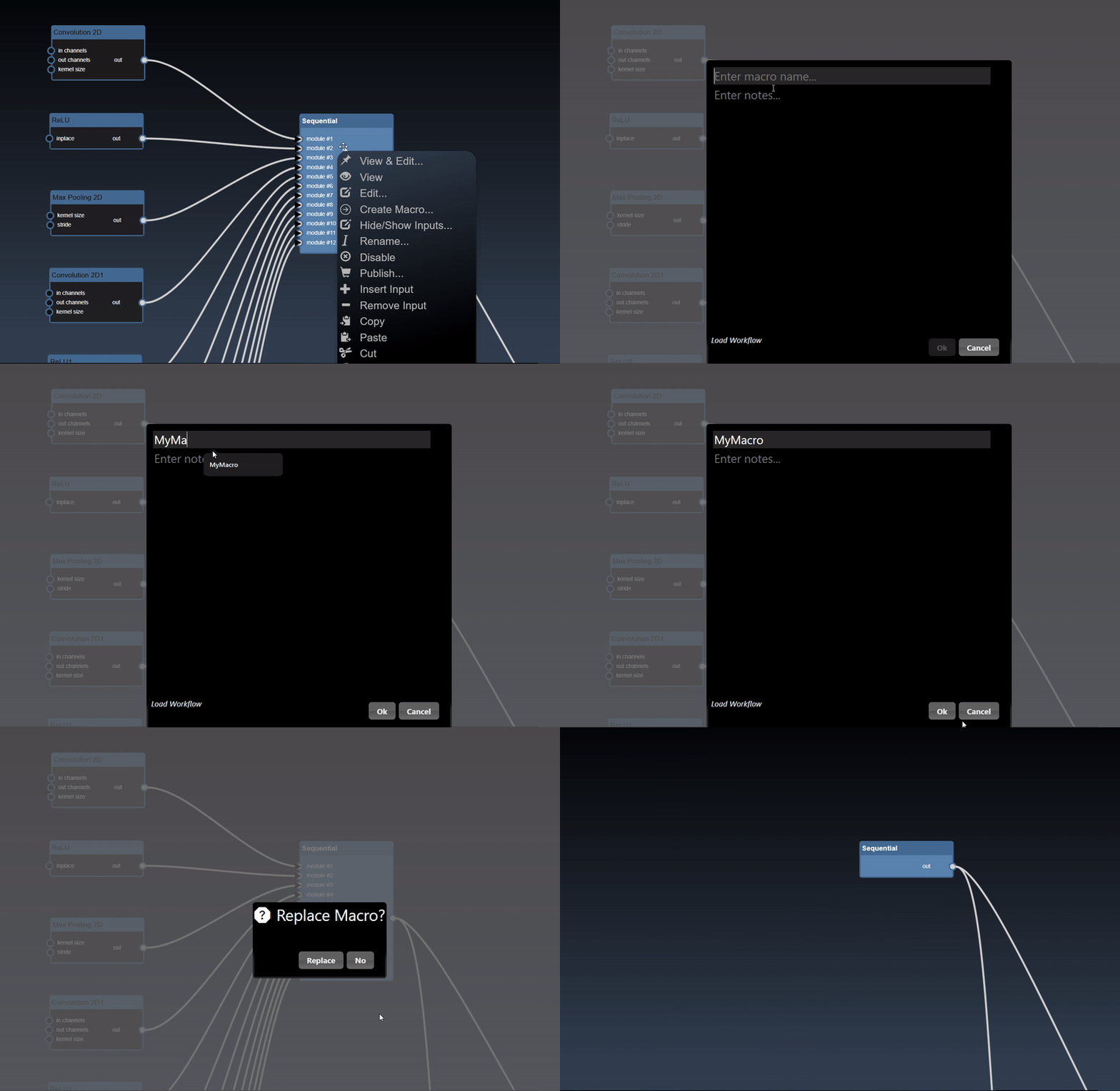
Create Macro: allows you to create a new tool by using the Create Macro UI
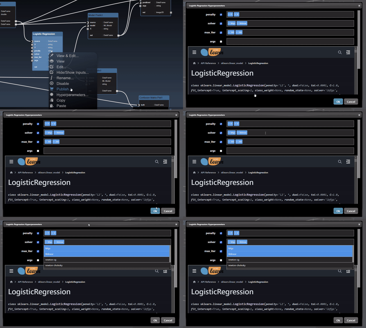
Hyperparameters: allows you to set the range of values on the hyperparameters of your model using the Hyperparameters UI
Grid Search: allows you to perform a grid search to optimize your model using Grid Search UI
Experimental
Copy URL: is available for viewer nodes that show the thumbnail of the image, the streaming URL of the image is copied to the system clipboard
Selection
When you bring up the context menu without a node selected, the flowgraphs viewport functions are shown:
Select All: allows you to select all the nodes in your flowgraph
Parameter Editor
The Parameter Editor allows you to edit the parameters of the currently edited node
The dialog is laid out as the tool icon and the name of the node being edited, followed by the list of that node's input parameters, and finally the dialog buttons.
Clicking the node's name opens a webpage with the tool's full description.
Only inputs that aren't already connected via the flowgraph show up as editable parameters here - a connected input's value comes from its upstream node instead.
Hovering over the parameter will show the description of the parameter:
The dialog buttons allow you to close the dialog - either you can accept the changes made by clicking OK, or reject any changes made to the
parameters by clicking Cancel. A button also allows you to Reset All the parameters to the original default tool settings.
The UI for each parameter input will be based on the type of the input, but all of them will have a reset icon that
allows you to reset that particular parameter input back to its default value. The different types of parameter UI controls are as follows
Numeric textfield
A numeric input allows you to enter a value. There are also step controls that allow you to increment one unit up and down.
Dragging below the numeric input reveals a range slider. While dragging, hold Shift for smaller step changes or Ctrl for larger ones.
For whole number and decimal parameters (not the multi-component numeric2/numeric3 versions), an icon next to the reset icon opens a
standalone calculator so you can compute a value with +, -, ×, ÷ and type it directly into the field.
Numeric2 textfield
Two numeric inputs allow you to enter both numerical values.
Dragging below the numeric input reveals a range slider. While dragging, hold Shift for smaller step changes or Ctrl for larger ones.
Numeric slider
A slider appears whenever the parameter declares minimum and maximum values.
While dragging, hold Shift for smaller step changes or Ctrl for larger ones.
Numeric2 slider
Two numeric inputs with sliders that can optionally be locked together to modify both values
at the same time.
While dragging, hold Shift for smaller step changes or Ctrl for larger ones.
Checkbox
A checkbox toggle for setting a true/false value
Selection menu
A dropdown menu for setting the value to one of a predefined set of choices.
Multi selection menu
Lets you add several values as tags. Click the widget to see the list of permitted values;
some multi-selection parameters also accept your own custom values outside that permitted list.
Textfield
A multi line textfield to allow you to enter the value for string parameters
Point
A point allows you to set the values with a textfield and also
has an icon that when clicked opens the viewer and you can select a point by clicking
in the image directly
Color
A color button when clicked allows you to set the color using a color dialog
Curve
An icon when pressed opens the bezier curve editor
Map
A map is a series of key/value pairs.
Clicking the widget opens a dialog editor that shows documentation and lets you enter each key/value pair
Filebrowser
An icon when pressed opens the IO Dialog that allows you to set the file location.
The prefix ${assets} is used to specify the file location is in the assets folder.
Tabs
Some tools lay out their controls across several tabs instead of one long list.
Viewer
Example: the real Viewer toolbar (hover any icon to see its name)
1:1|||
Hover any icon above to see its name. The divider groups are: zoom/inspection, frame playback, wipe compare, color channels & adjustments, and the collapsible More Tools menu (Measurement, Keystone, Stabilize, Multi-View, plus the Path Editor tools).
The viewer allows you to view the outputs of the currently viewed node
The viewer's toolbar includes the following functions:
Toggle Fullscreen: Switches the viewer between windowed and maximized view.
1:11:1 Pixel Zoom: Resets zoom so that one image pixel equals exactly one screen pixel.
Zoom In: Increases the magnification of the image.
Zoom Fit: Resets the zoom level to fit the entire image within the current window.
Zoom Out: Decreases the magnification of the image.
Resolution Information: Displays resolution, bit depth, and memory usage. Also lets you set the project resolution.
Toggle Border: Enables or disables a high-contrast guide border 1 pixel outside the image boundary. Useful for checking alignment against the canvas.
First Frame: Jumps to the start of the sequence.
Previous Frame: Steps back one frame.
Toggle Play: Starts or stops the sequence playback.
Next Frame: Steps forward one frame.
Last Frame: Jumps to the end of the sequence.
Set Current Frame: Opens a dialog to jump to a specific frame number.
Toggle Wipe: Activates Split Screen mode. Drag the divider to compare live view vs reference; drag the circular handle at either end to rotate the divider's angle.
Capture reference: Stores the current frame to be used as the reference image for the Wipe tool.
Color Channels: Isolate Red, Green, or Blue channels in grayscale. The White dot returns to full color.
Note: Active dots flash to indicate filtering.
Image Adjustments: Opens sliders for Gamma, Brightness, and Contrast. Settings reset when closed.
More Tools: A collapsible menu containing advanced utility tools:
Keystone: Warps a user-defined 4-point keystone in the video scene into a flat, rectangular image.
Stabilize: Allows tracking and 1 or 2 point stabilization.
Orbit: For a 3D scene node (Gaussian Splat Render), the mouse spins, zooms and pans its camera - see Orbit camera.
Multi-View: Compares the current view against up to 3 sources you add, live, side by side - see Multi-View.
Path Editor Tools
Insert Point: Places a single coordinate marker.
Insert Rectangle: Draws a 4-point rectangle.
Insert Ellipse: Creates a circular or elliptical region.
Insert Shape: Allows drawing of custom polygons by clicking.
Insert Freehand: Sketch a custom path freely with the mouse. (Long-press for Vector Brush thickness options)
Insert Lasso: Intelligent selection tool for defining shapes. (Long-press for Stroke envelope thickness options)
Convert to Bezier: Changes sharp corners into smooth curves.
Convert to Point: Changes smooth curves back into sharp corners.
Delete Selected: Removes the active point or shape.
Undo/Redo: Revert or repeat your last path editing actions.
The Viewer window, with its toolbar docked to the top of the canvas
A node can be viewed using the node context menu and selecting 'View' or 'View & Edit'. When viewing a node with multiple outputs a menu will ask which output to view, or double click the output port directly to skip the menu.
Zoom and pan with the mouse scroll wheel or a zoom gesture, then drag to pan. When zoomed in, a thumbnail of the full image is shown together with a slider to set the zoom amount.
Point parameters in the Parameter Editor can be set in the viewer. Select the overlay icon and then click in the viewer to set the location of the point.
Only one node can be viewed at a time in the viewer, but the flowgraph can show multiple node outputs at once via the 'Thumbnail Image Display' or 'Full Image Display' tools - maximize/minimize by hovering the corner and clicking . Additional Display Nodes are available too.
The viewer, on top of displaying images, has specific UI to display mutli-dimensional data:
Measurement Mode Buttons: A toolbar containing options to select tools such as Calibrate Quad, Ruler, Angle, Angle 2 Lines, Multi-Segment, Radius, and Diameter
Dynamic Instruction Label: Displays real-time, context-aware instructions depending on the active measurement tool and the current step of point placement
Calibration Settings Panel: Appears when homography mode is selected, allowing users to define the Plane Width, Plane Height, and measurement Units (e.g., mm)
Show Calibration Checkbox: Controls the visibility of the calibration quad and projected perspective grid lines
Measurements List Container: A scrollable summary view that lists all recorded measurements along with their calculated values and individual delete buttons
Keystone
Enable Keystone Warp Checkbox: Activates or deactivates the keystone correction effect
Instruction Box: Guides users on how to click and drag any of the four corner handles or click on the image to trace a new 4-point warp region
Reset Area Button: Instantly resets the keystone quad back to its default bounds (10% inset from the image edges)
Stabilize
Enable Stabilization Checkbox: Allows users to toggle stabilization on or off, which also manages video playback behavior
Tracking Points Selector: A dropdown menu allowing users to choose between 1 Point (Translation) and 2 Point (Scale & Rotate / Similarity) modes
ROI and Template Size Inputs: Editable number fields to configure the Region of Interest (ROI) size and template size
Tracking Execution Buttons: Circular buttons designed to trigger automatic Track Backward and Track Forward operations
Timeline Section: Features a range slider to scrub through frames, a real-time frame label indicator, and a calculator button that opens a custom on-screen numeric keypad for precise frame selection
Orbit camera (3D scenes)
When the viewer shows a node with a 3D camera, such as Gaussian Splat Render (cuda.gaussian_splat_render), an Orbit badge appears at the
top left and the mouse moves that node's camera instead of panning the picture. The node's inputs (yaw, pitch, distance, target) update live, and an open
properties panel follows.
Drag: spin the camera around its target (yaw and pitch)
Wheel: zoom (distance)
Right-drag or Shift-drag: pan the target
Double-click: back to the view the node had when it was opened
Orbit checkbox: off gives the viewer's normal pan and zoom back
The node also has a depth output (scene units per pixel, 0 where there is nothing) and a count output (splats in the scene). Its up_axis
input picks which way is up (scenes trained in the Digital Twin Studio use the default, -Y).
Multi-View
Multi-View compares up to 4 image sources live, in one place - a wipe divider or side-by-side split for 2,
a tiled 3-way or 4-way view for 3 or 4. Slot A always tracks whatever you're currently viewing in the main
viewer; slots B, C and D are added and removed manually from the Multi-View dialog itself, so browsing to
something else in the flowgraph never disturbs a comparison you've already built up. It never permanently
adds anything to the flowgraph: opening Multi-View creates a temporary, hidden compare node behind the
scenes, and closing Multi-View removes it immediately. Only image outputs can be compared this way (not
data frames, tensors, or other non-image views).
Multi-View entry: Found under More Tools - always available, even before anything else has been added.
Mode buttons:Wipe (antialiased draggable divider - drag the line to move it, the circular handles at each end to rotate it, same interaction as the regular Toggle Wipe tool), Split View (top/bottom split, no divider), 3 View (one on top, two side by side below), and Quad View (four quadrants). Only the modes valid for how many sources are currently being compared are enabled - Wipe and Split View both need exactly 2, 3 View needs 3, Quad View needs 4. In Split View, 3 View and Quad View, each tile briefly flashes its letter (A/B/C/D) whenever the layout appears or changes, so it's clear which source is which.
Comparing list: One row per source, labeled A/B/C/D. Slot A always shows the current view. Use the Add source row to fill B, C or D; each filled row (except A) has a remove button, so swapping a pick is just remove, then add again. When a row's source traces back to a playable video or camera node, a play/pause button also appears on that row to control it directly - closing Multi-View automatically resumes anything paused this way.
Add source picker: Opens with two tabs. List groups every node's image outputs under its node name, with a search box (filters by node or port name; Enter picks the match if the search narrows it to exactly one) - handy once the flowgraph has a lot of nodes. Diagram is a read-only, pan-and-zoom schematic of the flowgraph itself (drag to pan, scroll to zoom) - nodes with an image output are highlighted, and clicking one of their port dots picks it directly. In both tabs, a small green A/B/C/D badge appears next to any port that's already part of the current comparison, so it's easy to see what's already in use at a glance.
Multi-View is only available from the main viewer - it isn't part of the AI Label Studio or Video Segmentation Studio viewing workflow.
To watch many outputs at once rather than compare a few against each other, see Live Tiles, which replaces the
flowgraph with a grid of up to 16 live views.
Live Tiles
Live Tiles, on the App Menu bar and also under its Windows menu,
replaces the flowgraph with a grid of live node outputs - 2×2, 3×3 or 4×4, so up to 16 views at once. It is a switch, not a
window: the schematic and the Toolbox step aside while the grid is up, and come back when you close it. Opening Live Tiles also closes the
image viewer and the Parameter Editor, so the grid starts as the only thing you are looking at.
Where Multi-View compares a few image sources against each other, Live Tiles is for watching many at once -
and it is not image-only. Any viewable output port can go in a tile, including data frames, tensors and plain numbers.
Example: a 2×2 grid - the control strip across the top, two bound tiles, two empty
|171 / 4492×23×34×4
Movie Reader · out
Canny Edge Detector · out
The strip is the only chrome in tile mode. The button shows and hides the timeline - it is hidden by default, and
nothing is polled while it is hidden. The two buttons in a tile's top corner appear on hover - shown here on the first tile only:
opens that tile's Layers bar, clears the tile.
Each view is scaled to fit its tile, so a wide frame letterboxes rather than being cropped.
Filling a tile
Click an empty tile to open the port picker - a pan-and-zoom schematic of the flowgraph. Click a node to take
its output port; if it has more than one, a pie menu of its ports opens over it, with a hub to cancel (Escape or a
click outside also closes it). The port dots themselves are still clickable if you prefer to aim at one directly.
Drag a tool from the Toolbox onto a tile. An empty tile accepts a source - anything no image can be wired into, such as a
Movie Reader, Webcam, InfiniCam or Hawk. A tile that already shows something accepts any tool that can take what the tile shows, and the tool is
spliced into the chain rather than hung off it as a branch. A tile that cannot take what you are dragging says why, on the tile
itself - for example "needs image2D, this is matrix2D".
A tool that needs a file - a Movie Reader, for instance - opens the file browser on the spot. Pick the movie and it starts playing
in the tile; you are not sent back to the flowgraph to finish the job.
Drag one tile onto another to move its view there. If the target already holds something, the two swap.
Double-click a tile to leave the grid and open that node with View & Edit - the viewer and the
Parameter Editor together, exactly as double-clicking the node in the flowgraph does. A single click just selects the
tile's node, so the grid stays up.
Undoing a change
Undo and Redo on the strip cover the
workflow edits you make from the grid - adding a node, deleting a layer, reordering one. They are the application's own undo history, the same one the
Edit menu and Ctrl+Z use, so a change made in the grid can equally be undone from the flowgraph afterwards and
the other way round. Each button greys out when there is nothing to undo or redo.
What a tile is showing is not part of that history: binding a tile, changing the layout, or opening the layer bar are view settings, not
workflow changes, so Undo steps past them to the last real edit.
Layers
A tile shows one port, but the chain of nodes feeding it is usually what you actually want to work on. The button on a tile
opens the Layers bar, docked where the Toolbox sits and laid out left to right, source first - the same direction the flowgraph reads.
Example: the Layers bar for a tile showing Movie Reader → Canny Edge Detector → Brightness
Tile 12 layersfollow chain
Movie Reader
Canny Edge Detector
Brightness
The first card is the source the tile is anchored to - shown in italics, and never moved or deleted from here. The highlighted card is the
layer the tile is currently showing: marks what is being viewed and
what is open in the Parameter Editor - the same two glyphs the flowgraph puts on a node.
Click a card - anywhere on it - to show that layer in the tile and open it in the Parameter Editor.
Enable / disable the layer's processing, leaving it in the workflow.
Reorder - move a layer earlier or later in the chain. The
edges are rewired for you.
Delete the layer. The chain closes over the gap, so what fed it now feeds what followed it. A layer
whose removal would leave the rest of the chain unable to connect is disabled rather than allowed to break the workflow.
follow chain jumps the tile between the two ends of its chain - the source it is anchored to, and whatever it finally becomes.
The chain is the straight run of nodes feeding the tile: it stops at a fork and before a sink, and a node with more than one input - a blend, say -
starts the chain rather than continuing it, since everything before such a node fed only one of its inputs. Branching graphs are still edited
in the flowgraph.
What the grid costs, and what it keeps
Only bound tiles cost anything. An empty tile is free, and shrinking the layout releases the tiles that fall outside it rather
than leaving them running off-screen.
Closing the grid removes every view - it does not hide them. Nothing keeps encoding in the background once the grid is closed.
The grid is saved with the workflow. Which tile shows which port, and the layout, are stored in the workflow file, so they come
back when you load it again - including after restarting the application. The temporary view nodes themselves are never saved.
Importing a workflow replaces the grid. The imported workflow's own grid is loaded, or the tiles are emptied if it does not have
one. Bindings never carry over from the workflow you were just in, so you are never left looking at tiles pointing at nodes that no longer exist.
A tile whose node is deleted simply goes empty - the same as a tile that was never filled, ready to be
pointed at something else. It is not forgotten, though: if the node comes back, by undo or by loading the workflow again, the tile picks it up
where it left off.
Publishing the grid (phones and other computers)
Publish on the strip gives a link to a read-only view of the grid: the same tiles, live, with no
editing - just view. Open opens it in a new tab, Share uses the system share sheet (or copies the link where
sharing is not available) and Copy copies it. When the qrcode module is installed the popover also shows a QR code to
scan with a phone.
Made for phones. Tiles are fixed squares - one column on a phone, two on a tablet, the whole grid fitted to the window on a
computer - and the page has a Share button of its own for passing the link on.
Live only while Live Tiles is open here. Close the grid in InfiniWorkflow and the view shows Not live; it comes
back by itself when the grid is reopened.
Other devices need the network. By default InfiniWorkflow only listens on this computer, so the link opens here only. To view
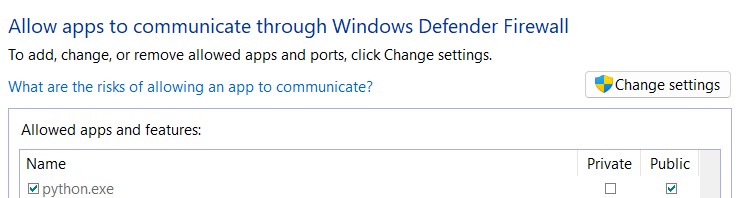
on phones and other computers, start InfiniWorkflow with -url 0.0.0.0 and allow its port (5000 by default) and the tile ports
8090-8093 through the firewall. The popover says which applies.
Anyone who can reach the computer can open the link - there is no sign-in on the view page, so publish on networks you trust.
Data frames
Dataframes represent 2D tables and are implemented using the Pandas Python module.
The viewer displays the DataFrame as a HTML table. Additional controls allow you to slice a set of the rows and columns, in the example below we slice rows [30-40).
The icon allows different views of the table including showing the sliced rows and columns,
with red cells represent missing data, a summary description of the statistics of each column, a line chart of the numerical
columns and the description of the types of each column:
Numpy Arrays
Numpy represents multidimensional numerical arrays and are implemented using the Numpy Python module.
You can set a matrix using the Set Matrix tool.
The viewer can display Numpy arrays in a variety of different visualizations where it will select the most useful
visualization first and by clicking the allows you to visualize other representations of the arrays.
Slicing controls are also available to reduce the tensor to a subset of its numerical data.
1D array (Set Matrix tool, numbers separated by spaces/commas/semicolons/tabs): viewed as a histogram, dot plot, line chart, or histogram chart
2D array (rows separated the same way): viewed as a heatmap, 3D height map plot, line chart, or table
3D array (comma-separated entries, each a number or a [] list): viewed as a 3D plot or a list of lists
Tensors
Tensors represent multi-dimensional numerical arrays and are implemented using the PyTorch Python module.
The viewer can display tensors in a variety of different visualizations where it will select the most useful
visualization first and by clicking the allows you to visualize other representations of the tensor.
Slicing controls are also available to reduce the tensor to a subset of its numerical data.
1D tensor: viewed as a histogram, dot plot, line chart, or histogram chart
2D tensor: viewed as a heatmap, 3D height map plot, line chart, or table
3D tensor: viewed as a 3D plot or an abbreviated tensor list
Image to Tensor: viewed as a 3D image, 3D height map plot, 3D color space plot, or abbreviated tensor list
Beyond displaying images and matrices, INFINIWORKFLOW has specific UI to display one-dimensional audio data:
Project Resolution
The concept of the project resolution is meant to be used for spatial parameters (points and path parameters).
These parameters will have defaults in percentages, for example a point parameter could have the deualt of (50%,50%),
which corresponds to the center of the project resolution. After nodes are placed down the defaults are converted to pixel
coordinates and the user will set pixel coordinates. However, you can change the project resolution and then also select
to modify the spatial parameters to also be updated. This allows the user to work in different resolutions but have the
workflow adjust to the new resolution if needed (this is also known as working in a "proxy" resolution, typically a
lower resolution but then later swith to the full resoultion for final processing.)
Path Editor
The Path Editor allows you to draw, modify, and manage vector-based shapes and paths over the viewer. These tools are primarily used for measurements, defining regions of interest (ROI), or masking.
Creation Tools
Insert Point: Places a single coordinate marker at the clicked location. Useful for pinpointing specific features.
Insert Rectangle: Creates a 4-point closed rectangular path. Click and drag or click corners to define the .
Insert Ellipse: Generates a circular or elliptical path, ideal for measuring rounded objects or apertures.
Insert Shape: The standard polygon tool. Click to place vertices; the path will automatically close if you click the initial point.
Insert Freehand: Allows for organic path creation by following the movement of your cursor while the mouse button is held down. Supports Vector Brush mode (long press to select brush thickness).
Insert Lasso: An intelligent selection tool that helps wrap complex shapes by detecting edges or following specific mouse gestures. Supports stroke-envelope drawing (long press to select stroke thickness).
Modification & Geometry
Convert to Bezier: Transforms sharp linear segments into smooth curves using control handles for high-precision curvature.
Convert to Point: Reverts smooth Bezier curves back into sharp, linear corner points (polygonal vertices).
Editor Management
Delete Selected: Removes the currently highlighted point or the entire active shape from the canvas.
Undo: Reverts the last action performed in the path editor (e.g., a moved point or a newly added vertex).
Redo: Re-applies the action that was just undone.
Advanced Path Editing
Insert Shape (Polygons & Curves)
The Shape tool is used for creating both sharp-edged polygons and smooth, complex curves.
Click: Places a standard linear point (corner).
Click & Drag: If you hold the mouse button down and drag while placing a point, Bezier control handles will automatically extend from the vertex. This allows you to create curved segments in real-time without needing to convert the point later.
Vector Brush & Stroke Mode
The Insert Freehand and Insert Lasso tools support an advanced Vector Brush / Stroke Mode. Instead of always generating solid, filled shapes, this mode allows you to draw strokes and outlines of a specific thickness following your hand path.
Activating Brush Mode: Long-press (click and hold for 450ms) on either the Insert Freehand () or Insert Lasso () toolbar buttons to open the Brush Flyout Menu.
Brush Options:
Filled Shape: (Default) Draws a standard closed, solid-filled vector shape.
Small Brush (2px): Draws a thin 2px vector stroke envelope.
Medium Brush (6px): Draws a medium 6px vector stroke envelope.
Large Brush (10px): Draws a thick 10px vector stroke envelope.
Visual Indicators:
When a brush thickness greater than 0px is active, the Insert Freehand icon dynamically updates from a pencil () to a brush ().
An active tool with a custom brush thickness will be highlighted with a distinctive blue active-ring indicator in the toolbar.
Stroke Envelope Generation: When drawing with a non-zero brush thickness, the path editor automatically generates a closed polygonal boundary (a stroke envelope) representing the thickness of your stroke rather than just connecting the start and endpoints as a solid polygon.
Selection & Grouping
Managing multiple points is essential for complex adjustments.
Alt + Shift + Click/Drag: Holding Alt and Shift allows you to draw a selection marquee (box) around multiple points or click individual points to add them to your current selection group.
Shape Transformation Mode
When you have selected all points in a path (or a specific group of points), the editor enters Shape Mode.
The Bounding Box: A rectangular frame will appear around the selected points with handles at the corners and sides.
Moving: Click and drag anywhere inside the bounding box to move the entire shape as a single unit without changing its proportions.
Resizing: Click and drag the corner handles to scale the shape. Holding Shift while resizing will maintain the aspect ratio.
Pro-Tip:
To quickly enter Shape Mode for a single object, you can often double-click a segment of the path to select all connected vertices instantly.
Quick Tips:
Selection: Click on an existing point to select it; its color will change to indicate it is active.
Dragging: You can drag individual points to refine a shape even after the path is closed.
Keyboard Shortcuts: Use Ctrl + Z for Undo and Del for deleting selected points.
Photron High Speed Cameras
INFINICAM and HAWK are high-speed streaming cameras capable of capturing and transferring 1.2-megapixel of image data to PC memory at 1,000fps via USB 3.1. Infiniworkflow, on top of all of its many other functionalities, is designed to be a platform for using INFINICAM(s) and HAWK(s) and saving their footage. There are certain differences between nodes related to INFINICAM/HAWK and most other nodes, so if you will be using an INFINICAM or HAWK, reading through this section is the fastest way to understand everything Infiniworkflow can do with your camera.
1. INFINICAM / HAWK Viewer node:
When an INFINICAM or HAWK is plugged in, a node called "Infinicam" will come up. This node allows you to view the camera feed, and also set the preroll and postroll frames (pre/postroll frames will be discussed later). If multiple cameras are connected, each one will show up as its own node (i.e. "Infinicam", "Infinicam #2", etc). Note that the camera may take a few seconds to open. Also note that this node only allows you to view the feed; saving is done separately.
2. INFINICAM / HAWK Saving nodes:
Infiniworkflow has 2 ways of saving footage for each camera line — "Infinicam Save Movie" and "Infinicam Save Compressed" for INFINICAM cameras, and "Hawk Save Movie" and "Hawk Save Compressed" for HAWK cameras. These saving nodes will come up for each respective camera that is connected to your machine (in other words, if you have 2 INFINICAM cameras connected, "Infinicam Save Movie" and "Infinicam Save Compressed" save footage from the first, and "Infinicam Save Movie #2" and "Infinicam Save Compressed #2" save footage from the second — the same numbering convention applies to HAWK nodes). Note that these saving nodes do not need to be connected to the viewer node itself; all that is required is that the Trigger is clicked.
The "Save Movie" nodes ("Infinicam Save Movie" / "Hawk Save Movie"), upon hitting the Trigger, save footage from the selected camera in any file type (.MP4, .MDAT, etc.) and to any file location. The total number of frames that will be saved when the Trigger is clicked is based on your camera's pre-roll and post-roll number of frames. To explain what these terms mean, consider the following example: you wish to save footage whenever an object falls off a conveyor belt in a factory. You have a workflow that will set a Trigger to True as soon as it detects that an object has just begun to fall off the belt. To understand why objects sometimes fall off the belt, you want to save the 2000 frames of footage from before the moment the object begins falling, as well as 1000 frames of footage after that point for good measure. Thus, you will set your pre-roll to 2000, and your post-roll to 1000. When the Save Movie node is Triggered, a total of 3000 frames will be saved precisely as you want them to.
The "Save Movie" nodes tend to be slower, as they need to compress and decompress data on the fly. The "Save Compressed" nodes ("Infinicam Save Compressed" / "Hawk Save Compressed"), on the other hand, save out compressed images, which means footage gets saved to your computer faster and is more informationally dense (a single 2 second video can be a few hundred megabytes). Whereas the Save Movie nodes allow users to select the Codec and File format, the Save Compressed nodes hardcode both, so 2 files are always returned: a MDAT file of the footage itself and a CIH file of the footage metadata.
Note for all saving nodes: if the Trigger has already been pressed and you wish to stop saving (i.e. save a shorter clip of footage), you can simply click the Trigger again to immediately save out all frames already gathered to your machine.
If you wish to view footage saved from either "Save Compressed" node, use the "Infinicam Movie Reader" node, which reads MDAT/CIH files.
Important note: by default, when a "Save Compressed" node is Triggered, the number of frames saved will equal the camera's preroll plus postroll. However, if you wish to save footage continually, you can click the checkbox in the editing menu for "Constant Saving". When true, you may set the maximum file size for the saved footage. When the node is Triggered, footage will continue to save into the file you created until the maximum file size limit has been reached.
When 3 or more INFINICAM/HAWK devices are connected, additional nodes called "Infinicam Trio" and "Hawk Trio" become available in the catalog (both work identically - INFINICAM and HAWK devices are the same underlying camera pool in Infiniworkflow, so which one you see depends only on which brand name you drag onto the canvas). A Trio node drives three devices as one synchronized unit and packs them into a single 3-channel image - the Left camera becomes the Red channel, Middle becomes Green, and Right becomes Blue. All three cameras share one settings panel (fps, shutter, resolution, expose); there is no way to give the three cameras different acquisition settings, by design.
Which three physical cameras play the roles of Left/Middle/Right is chosen once, in a picker dialog, the moment you drag a Trio node onto the canvas - drag each detected camera tile into a Left/Middle/Right slot, then confirm. This assignment is then locked for the lifetime of that node: to point the node at different cameras, delete it and drag a new Trio node onto the canvas to pick again. This mirrors how a regular Infinicam/Hawk node's device cannot be changed after it is placed either.
Trio nodes require monochrome cameras - a device reporting a color sensor is refused with an error naming that device. The Left camera is automatically the synchronization (genlock) master; Middle and Right automatically slave to it. If the three cameras' frames ever drift out of alignment (a dropped frame, a disconnected cable), the node holds its last good composite and reports a sync-degraded status rather than silently showing a misaligned image.
Besides its main packed-RGB output, a Trio node has a second output called "strip", showing the three source frames laid out side by side (Left | Middle | Right) rather than merged into channels - useful for monitoring what each individual camera sees. This is only computed while something is actually connected to or viewing that output, so leaving it unused costs nothing.
Saving a Trio composite works the same way as a regular Infinicam/Hawk: connect (or simply enable) an "Infinicam Trio Save Movie" or "Hawk Trio Save Movie" node and click its Trigger. It saves the packed RGB composite as a normal color .avi/.mp4 (with the same preroll/postroll behavior described above for the single-camera Save Movie nodes), or as a single still .png image - there is no "Save Compressed"/MDAT equivalent for Trio, since a software-composited RGB frame has no camera-native compressed form to preserve.
If no INFINICAM/HAWK hardware is connected on a development machine, both the regular viewer nodes and the Trio nodes fall back to a simulated noise feed (clearly labeled "SIMULATED" on the image) so workflows remain buildable and testable without hardware attached; this simulated fallback never occurs on a production install.
Utilities
Audio
Audio is represented by a list of numerical intensity values over time and they are implemented using the Numpy Python module.
You can get audio using the Read Audio tool for audio files or the Input Audio tool for streaming input through the microphone.
The viewers in Audio nodes can display audio arrays in two different ways: a waveform and a spectrogram.
It will default to the waveform visualization first, which shows the loudness of the sound at every sample over time.
By clicking the , it allows you to cycle through visualizations.
The other visualization is a spectrogram, which is a colormap of frequencies over time where colors represent the volume of each frequency in decibels (dB).
Widgets
A set of tools, called Widgets, are available that provide user interface controls directly in the flowgraph
These widgets are an easy way to modify the parameters without having to open the Parameter Editor - you can
selectively decide which parameters are important enough to add as widgets to the flowgraph. For example, the following
flowgraph has a number of widgets added: a "Filebrowser Widget", a "Selection List Widget" and a "Slider Widget" are added to the
flowgraph as well as two "Output Widgets":
The Widget Note tool adds a sticky note to the flowgraph for comments and reminders. Type straight into it; drag it by its yellow title strip,
and click the title to rename it. Drag the folded bottom-right corner to resize it. The text and size are saved with the workflow.
Notes stay visible when you zoom far out, and Auto arrange leaves them where they are.
You can now modify those controls directly in the flowgraph. You can refine how each widget is shown by editing it in the
Parameter Editor and setting its widget attributes. Widget attributes include the name which will show for each
widget. Widgets such as Sliders allow you to set their specific attributes such as the minimum, maximum and step value for the Slider widget.
All widgets have the common attributes of the name and description (used for tooltips) as well as layouts. The layouts allow you to specify an optional
Tab that the widget will be placed in and also the order in which the control will be ordered in the UI (a lower order will allow the control at the top of the
layout). An example of the Widget Slider's parameters are as follows:
See the reference section for the full list of Widget Tools
Displays
A set of tools, called Displays, are available that provide viewing displays directly in the flowgraph
This allows you to constantly monitor the output of multiple nodes and avoid switching back and for using the Viewer.
Thumbnail Image Display: shows a node's image output
Full Image Display: shows the image at actual pixel resolution
Matrix2D Display: shows a matrix2D output as a table
DataFrame Display: shows the first few rows; double click for statistics/datatypes views
Tensor Display: double click for its other tensor visualizations
Displays are also available for ints, doubles, booleans, etc. for realtime output visualization
Map Display shows a map (JSON) as a collapsible tree.
See the reference section for the full list of Display Tools
Creating Triggers
You can create triggers to activate certain nodes that require the trigger to start execution. Typically, you can use the various boolean expression - for example,
in the workflow below, the number of detected faces is applied to a "Numeric a>b" tool, this will yield a true value whenever the number of faces is greater
than a certain amount. The output of this node is a "trigger" that is used to execute the "Text to Speech" node.
Automatic trigger: a "Numeric a>b" node compares detected faces against a threshold, its true output triggering "Text to Speech"
Manual triggers: the Widgets "Widget Bool Trigger" (binary pulse) and "Widget Int Trigger" (staircase function) can trigger one or several nodes by hand
Loop Triggers
Loop Triggers is allows you to update a Trigger Variable based on when downstream Python nodes have executed and trigger an upstream Python node.
This allows you to do "for" loops as the workflow graph is acyclic - meaning no edges can connect a downstream node to an upstream node, so loops are not allowed.
However, with this feature you can make a trigger happen upstream when a downstream node is executed. You can add two new nodes, 'Loop Variable' and 'Loop Trigger':
The Loop Trigger when the source has changed (or you click the next trigegr), will use the referenced Loop Variable and will trigger the output of the Loop Variable.
The Loop Variable can be placed upstream and flow back to the Loop Trigger, and thus this forms a loop cycle.
You can use Loop triggers to perform simulations which may require multiple passes of the workflow nodes.
Data Science
The Data Science tools are all under the Data Frame category.
The implementation is based on Pandas, an open source data analysis and manipulation library.
A DataFrame can be loaded with the "Read CSV" or "Read Excel" tools or created programmatically with the "Random Table" tool or converting from
numpy or tensors. For many of the tools, they will use "Column" or "Columns" properties representing a choice of a single column or a subset of columns.
Some of the tools also have an "arg" property which is a map parameter that allows you to pass in additional key/value pair optional arguments
The Key/Value Dialog UI will show the corresponding Pandas function's documentation which is useful to determine the additional parameters you wish to set.
A number of tools are available to create charts for DataFrames. These tools are all under the Plot category.
Each plot tool has parameters placed into two different tabs: Data and Layout.
The Data parameters allow you to set the columns you wish to plot and the Layout parameters allow you to adjust the title of the chart etc.
For example, the "Line Plot" tool has the following Data parameters. The X and Y allow you to set the columns you wish for the X and Y-axis. If no
columns are set for the Y-axis then the plot will include all numerical columns in the DataFrame. If the X parameter is not set then the index of
the DataFrame will be used as the X-axis.
In this example, two columns (sbp and tobacco) are plotted for Y against the "row.names" column.
The Layout tab allows you to specify the title for the chart as well as the labels for the axis. You can also hide or show the Legend and
set the size of the figure in inches. The "color" parameter is a multi-selection list parameter that you can set colors such as "red", or #6580ab
etc. If you have two Y columns you plot then if you set one color both line charts will use the same color but if you set two colors in the list
then you can distinguish each line chart.
An subset of the plot tool visualizations are as follows:
Histogram
Bar
Density
Hexbin
Line
Scatter
See the reference section for the full list of Plot Tools
Machine Learning with scikit-learn
The Machine Learning filters are based using scikit-learn Python module
are all under the ML category.
Each ML tool has 3 tabs: Train, Hyperparameters and Export. The Train parameters allow you to set the X and Y columns as well as a trigger to start the training.
Since training can be slow, a trigger is used to start the process - though when running a grid search, that trigger is generated automatically.
An example of the training parameters for the 'Logistic Regression' ML Tool. In this scenario, we are training a model based on the tobacco column to predict heart disease (chd) - clicking the "train" trigger starts the process of fitting the data to create an ML model.
The Hyperparameters tab has the specific hyperparameters that allow customization and tuning of the model - shown here for the logistic regression tool. Each ML training tool will have a different set of hyperparameters, and these will show up in the Grid Search dialog.
An "arg" map parameter is also included which allows you to set any parameters that are not in the UI - this is a map of key/value pairs. After clicking the "arg" widget, the Key/Value dialog appears showing the documentation of the ML model, useful to review any additional parameters you may wish to set.
The Export tab lets you set whether to save the model to a file - by default models are not saved, but it's recommended to save complex models that take time to execute. A common practice during grid search is to connect the "Is Batch" tool to the model's "save" input, so models are saved during the grid search process.
The typical approach to building models involves splitting your training data into test and train splits.
The following workflow illustrates the steps involved and the nodes
required to implement the training:
The CSV file is read and then a test train split is done, the training table is then passed to the ML model.
In this case the "Is Batch" Tool is used to set the "save" parameter which
will automatically save the model for any Grid Search. The output of the model is then passed to a model predict
and the predicted values can be compared against the ground truth
to establish the accuracy of the model. In this scenario, we use a confusion matrix to plot the accuracy of the results.
And a ML metric nodes such as "R2 Score" allow you to see the accuracy
and it can be further used to initiate a Grid Search.
See the reference section for the full list of ML Tools
Jupyter Notebook
The Jupyter Notebook node (Utilities) runs Python cells in a real Jupyter kernel,
one kernel per node. Cells can read the node's inputs, call every MCP tool of the running workflow, and send typed
values out of the node - so a notebook can be a quick experiment, a custom processing step, or a script that builds and inspects the workflow itself.
It needs the notebook package (see Downloadable Packages); calling MCP tools also needs the mcp package.
Ready-made examples are in the Notebooks demo folder: MCP Workflow Builder, MCP Inspector, Draw with OpenCV, Image In/Image Out,
Pixel Statistics, Pandas Speed Analysis, Matplotlib Chart, NumPy Signal FFT, Camera Config as Map, Typed Multi-Output, Math Chain,
Notebook to Notebook, Color Palette Extractor, Edge Density Map, Histogram Equalize and Workflow Report.
Opening a notebook
Double click the node: View & Edit opens as for any node and the notebook opens straight away
(the same as pressing its open parameter, which is in the parameter editor only, not on the node). With several outputs, pick one from the port menu first.
The dialog closes with or Esc - clicking outside it does not close it.
The run trigger on the node runs every cell in order without opening the dialog, stopping at the first error; the last cell sets the output,
exactly like Run all. Press it on the node, or connect a trigger to it.
Otherwise cells run only from the dialog. When the graph renders, the node sends its last saved result again without running any code,
so opening a workflow never executes notebook code.
Cells and toolbar
Shift+Enter runs a cell and moves to the next (adding one at the end), Ctrl+Enter runs it and stays.
Each cell has run, / move and
delete; Add cell is below the last one.
Toolbar: Examples (insert a ready-to-run cell),
run all, interrupt, restart the kernel
(clears all variables), import, export and run history.
Outputs show inline: printed text, errors with their traceback, values, tables (pandas DataFrames and numeric numpy arrays), images
(OpenCV/numpy image arrays, PIL images, matplotlib figures and plots). A cell that succeeds silently - an import, say - shows
Done in 0.02s.
Run history keeps every run with its time, code, output and duration; puts an old run
back as a new cell. Cells and history are saved with the workflow.
Import / export: export writes a standard Jupyter .ipynb with the cells and their outputs; import reads an
.ipynb (markdown cells come in as comments) or a .py file split into cells at # %% lines.
Interrupt stops normal Python code within a second or two. A single long call into C code (for example one
time.sleep(30)) cannot be interrupted on Windows - use restart instead.
Completion and help
Type mcp. and a menu of every MCP tool appears with its arguments; keep typing to narrow it, use the arrow keys, and
Enter or Tab to insert. The panel beside the menu shows the highlighted entry's documentation.
Tab after any name completes it (Python names, modules, attributes); Tab at the start of a line indents;
Ctrl+Space opens the menu anywhere.
Typing (, or Shift+Tab inside the brackets, shows the call's signature and documentation.
Calling MCP tools
The mcp object calls the same MCP tools an AI agent uses, directly on the running app: mcp.tools() lists them and
mcp.help("add_node") describes one. Results that are JSON come back as Python dicts and lists, and images from
mcp.get_node_image(...) show inline.
dag = mcp.get_workflow_json()
[v["name"] for v in dag["vertices"]]

blur = mcp.get_unique_node_name("Blur")
mcp.add_node("cv.blur", blur)
mcp.set_parameter(blur, "ksize", "15,15")
Inputs, outputs and types
The first output, out, is the value of the last cell (or what it printed, if it has no value); running the last cell
updates it, and an error leaves the previous value in place. After each run the port takes the value's type and the real value -
not a string - goes to the connected nodes. Links the new type cannot feed are removed, and the dialog says so.
Last cell value
Output type
OpenCV/numpy uint8 image, PIL image, matplotlib figure or plot
More ports are added with the node's + buttons (see Adding and Removing Ports); each one asks for its type.
Inputs can be any, int, double, string, map, image2D, matrix2D or DataFrame; outputs can be one of those types or auto, which
follows the value like out does. A bar at the top of the dialog lists the ports - click one to insert the code for it.
img = get_input(0)          # or get_input("in 1") - images arrive as OpenCV BGR arrays
n = get_input(1)            # numbers as int/float, maps as dicts, tables as DataFrames
print(inputs)               # lists the inputs

set_output(1, table)        # the output after out ("out 2"); checked against its declared type
set_output("out 3", {"fps": 20000})
NODE holds the notebook node's own uuid. Types, links and each output's last value are saved with the workflow, so a reopened
workflow sends the same typed values without running anything. The values are kept in ${assets}/.notebook_results; on another machine
they appear after the cells are run there.
Map type and Map Display
A map is a JSON object (a Python dict). It is output by Set JSON, JSON File Reader and notebooks,
and read by the Get JSON nodes. A map can connect to any string input - it arrives as its JSON text - and a JSON string can connect
to a map input. Viewing a map shows it as a collapsible, colour-coded JSON tree, and the Map Display
shows one directly in the flowgraph (see Displays).
Shadertoy
The Shadertoy node (Experimental) runs a GLSL fragment shader pasted from
shadertoy.com live on the GPU. Copy the code of a shader's Image tab
(its mainImage(out vec4 fragColor, in vec2 fragCoord) function) into the node and it runs on every frame, animated by iTime.
It uses OpenGL like the other GPU shader nodes, so it is Windows only; connect a Texture Upload in front of it, as in the demos.
Ready-made examples are in the Shadertoy demo folder: Water Ripple, Retro CRT, Kaleidoscope, Neon Edges, Glitch, Thermal Camera
and Comic Halftone. Double click the Shadertoy node in a demo to see its output and its code.
The code editor
Double click the node: View & Edit opens as for any node, together with the code editor beside the viewer, so the result
stays visible while you edit. The edit button in the parameter editor opens it too.
Apply (or Ctrl+Enter) saves the code into the node and compiles it. A compile error
is shown under the code with its line marked in red in the margin; the last shader that compiled keeps running until the error is fixed.
Examples... loads one of the built-in shaders (Plasma Overlay, Water Ripple, Retro CRT, Kaleidoscope, Neon Edges, Glitch,
Thermal Camera, Comic Halftone and the shadertoy.com starter) and applies it.
Tab indents (Shift+Tab outdents a selection), Enter keeps the indentation, and Esc or
closes the editor. Drag its title bar to move it and its corner to resize it.
What the shader can use
iChannel0 is the incoming frame and iChannel1 the optional second input; both are read with texture()
the right way up, with shadertoy.com's bottom-left origin for fragCoord.
iResolution is the frame size, and iTime, iTimeDelta, iFrame, iDate and
iMouse are provided (iMouse only changes in the native GL viewer window). The speed parameter scales iTime; 0 freezes it.
Single-pass shaders work. Shaders that need Buffer A-D tabs, sound, cube maps or keyboard input are not supported.
Tools
Actions
Workflow functions called directly in-process - no LLM, no network, so they run in milliseconds. These tools are all under the Actions category. The full list of display tools is as follows:
Agents
Launches a real Claude CLI subprocess with its own MCP access to the workflow - output depends on model judgment, not a fixed function. These tools are all under the Agents category. The full list of display tools is as follows:
AI
AI Inference algorithms including using pretrained models. These tools are all under the AI category. The full list of display tools is as follows:
Audio
Audio signal processing filters. These tools are all under the Audio category. The full list of display tools is as follows:
Color
Image Color Correction filters. These tools are all under the Color category. The full list of display tools is as follows:
Composite
Combine and Split Images. These tools are all under the Composite category. The full list of display tools is as follows:
Database
Database processing such as reading tables, performing queries and writing to databases. These tools are all under the Database category. The full list of display tools is as follows:
Datascience
Datascience filters using the Pandas library. These tools are all under the Datascience category. The full list of display tools is as follows:
Experimental
Experimental Tools. These tools are all under the Experimental category. The full list of display tools is as follows:
ImageProcessing
Image Processing Filters such as Blurs, Edge Detetors and Morphological Filters. These tools are all under the Image Processing category. The full list of display tools is as follows:
Grayscale
Grayscale Filters that create single channel images. These tools are all under the Grayscale category. The full list of display tools is as follows:
Hugging Face
Run models from the Hugging Face Hub: type a model ID and it downloads and runs. These tools are all under the Hugging Face category. The full list of display tools is as follows:
Inputs
Source Inputs such as Webcameras or Reading Movies. These tools are all under the Inputs category. The full list of display tools is as follows:
Live
Feed dashboards, sheets and documents: log workflow results over time and export boards to PDF. These tools are all under the Live category. The full list of display tools is as follows:
Logic
Logical functions for conditional processing, useful to create triggers. These tools are all under the Logic category. The full list of display tools is as follows:
Math
Mathematical and Scientific Operators. These tools are all under the Math category. The full list of display tools is as follows:
Matrix
Matrix operations using numpy arrays. These tools are all under the Matrix category. The full list of display tools is as follows:
ML
Machine Learning filters based using scikit-learn. These tools are all under the ML category. The full list of display tools is as follows:
Outputs
Display tools that allow you to visualize directly in the flowgraph. These tools are all under the Outputs category. The full list of display tools is as follows:
Photron
Photron Camera and Processing Tools. These tools are all under the Photron category. The full list of display tools is as follows:
Plot
Plotting tools using Matplotlib. These tools are all under the Plot category. The full list of display tools is as follows:
Pytorch
PyTorch deep learning for building ML models. These tools are all under the Pytorch category. The full list of display tools is as follows:
Recall
Knowledge from documents and footage: index files into a library, then ask questions and get answers that cite the page or the moment. These tools are all under the Recall category. The full list of display tools is as follows:
Rendering
3D tools to create 3D scenes and render. These tools are all under the Rendering category. The full list of display tools is as follows:
Statistics
Image Statistics tools such as mean, median and RMSE. These tools are all under the Statistics category. The full list of display tools is as follows:
String
String tools such as string concatentation. These tools are all under the String category. The full list of display tools is as follows:
Tracking
Tracking features in images. These tools are all under the Tracking category. The full list of display tools is as follows:
Transform
Image Transformation tools. These tools are all under the Transform category. The full list of display tools is as follows:
Triggers
Triggers tools which are useful to create signals for control. These tools are all under the Triggers category. You can create triggers to activate certain nodes that require a trigger to execute - review the section Creating Triggers. The full list of display tools is as follows:
Utilities
Python Utility tools. These tools are all under the Utilities category. The full list of display tools is as follows:
Verticals
Industry-specific tools spanning agriculture, robotics, medical, logistics and more, each tagged with the vertical it belongs to. These tools are all under the Verticals category. The full list of display tools is as follows:
Widgets
User Interface Widgets which can be used for Publishing a simplified UI. These tools are all under the Widgets category. The full list of display tools is as follows:
System Performance
The "System Performance" tool can be used to report performance metrics of your workflow. You can add it to your
workflow and it will output a table of counters that will refresh regularly to show the performance for each node.
The output table format is described below:
Column
Description
name
Name of the node
Work(ms)
Average time in milliseconds to process one frame
#Wait
Number of times since last update the node waited because inputs were not ready or hadn't changed
#Render
Number of times since last update the node executed
Host to Host(MB)
Amount of System CPU Host memory copied in megabytes
Host to Device(MB)
Amount of System CPU Host memory uploaded to the GPU memory in megabytes
Device to Host(MB)
Amount of GPU memory to the System CPU Host memory in megabytes
Device to Device(MB)
Amount of GPU memory copied in megabytes
Peer to Peer(MB)
Amount of GPU memory in megabytes copied between different GPUs when multiple GPU are available on the system
Sheets, Dashboards & Documents
Analytics > Sheets / Dashboards / Documents (the chart icon next to Windows on the top toolbox) turn what your workflow measures into a spreadsheet, a live dashboard and a
signed report. A sheet is a workbook with tabs and Excel-style formulas; use the sheet's Workflow toolbar (Live value, Live picture, Live table for matrix / DataFrame outputs that fill right and down from the cell, History, Parameter, From results) or right-click a cell and choose Bind to workflow output… to pick a node's
output port on the schematic, and the cell shows its value (or a refreshed thumbnail for pictures) live, as =IW("Node", port). A live value can
also keep its last N values (=IW.HISTORY), which spill into a range you can chart, pivot and use in formulas; the History button opens a wizard (what, how many, how often, layout, extras) so no formula is needed, and fx next to the formula bar inserts any function with a live preview. Dynamic-array formulas (FILTER, SORT, SORTBY, UNIQUE, SEQUENCE, TAKE, DROP) spill into the cells below as in Excel 365, and A2# refers to the whole spilled range. A dashboard shows sheet cells,
logged results or node outputs as KPI tiles, charts (chosen automatically from the data), gauges, heat maps and live cameras; click a chart to filter the
whole dashboard or to jump the viewer to that moment, and set alerts and scheduled PDF reports. A document is a report page with live blocks; the final
sign-off freezes every value and picture into a signed version. All three are saved inside the workflow (use Save Workflow), export as
.iwboard.json, and print to PDF; documents also export to and import from Word (.docx), and sheets open and save Excel workbooks (.xlsx) with their formatting. Suggest from this workflow proposes a sheet or dashboard from the workflow's outputs.
Sheet charts include combo (bars + line, with a right axis when the scales differ), scatter, histogram, box plot and waterfall, with linear, moving-average or exponential trend lines (R² on request) and forecasts (Holt-Winters or linear, dashed with a 95% band).
Answers from a Recall library can sit next to the data: see Recall in dashboards, documents and sheets.
See the full Sheets, Dashboards & Documents guide; scripts and AI agents use the sheet_*, dashboard_*
and document_* tools on the MCP page.
Stories: a dashboard's More menu builds a slide-style story from its blocks (up to 4 per slide, each with a caption), shown full screen
with the arrow keys and printed to PDF one slide per page. A slide can stay live or be frozen at the current values. See
Stories.
Recorder: the red Record button in a dashboard's toolbar opens the Recorder drawer. It keeps what the dashboard is watching in a memory
ring buffer on IW's server (not in the browser, so it keeps going when the tab is closed): camera / picture tiles as frames (at the tile's rate,
10 fps by default), matrix / table tiles as rows with their column names, and number tiles as values (tiles reading the results store are read
back from it when saving). The buffer is bounded by the max duration and a memory budget (the oldest samples are dropped first).
A trigger decides which slice is kept, as on a Photron high-speed camera: Start keeps max duration from the trigger, Center keeps
the set seconds before and the rest after, End keeps the last max duration up to the trigger, and Manual records from
Record to Stop & save (it stops by itself at the max duration). Arm starts buffering; the trigger is Trigger now,
a tile value crossing a limit for a hold time (the same operators as Alerts), a new event of a type in the workflow's events table, or a daily time.
With Re-arm after saving, a hold-off stops a flapping condition from making a clip every few seconds. Tiles being recorded show a
REC badge. Each recording is saved in ${assets}/recordings/<workflow>/<dashboard>/<date>_<time>_<reason>:
an MP4 (or WebM) per camera at the recorded rate (a demo movie file is cut frame-exact straight from the movie), one CSV per matrix tile
(t, time, frame, row and the named columns), values.csv (one column per value tile and a trigger mark), an optional
dashboard PDF at the trigger, trigger.json and manifest.json. The drawer lists the recordings with their size and files;
open their folder or delete them there. Scripts use the dashboard_record_* MCP tools.
Digital twin tiles: two dashboard tiles turn a 3D scan from the Digital Twin Studio into a live site view, both bound to a
Gaussian Splat Render node. 3D view (splat_view) is the node's live picture: drag to orbit, the wheel zooms, the house button resets.
Site map (splat_map) is a top-down map made from the scan (cached next to the .ply), with the path the capture walked, the 3D
tile's view as a cone, and a numbered pin per live camera with its direction. Click the map to move the 3D view to that spot (the camera comes in from the
nearest point the capture covered, where a scan looks sharp), drag to choose which way it looks, and click a camera pin or its chip to open that camera's live
video and turn the 3D view to the camera's own viewpoint; Overview returns to the opening view. Both tiles share one camera, so orbiting in 3D moves
the cone on the map. A camera's pin needs its pose in the scan (the view that matches its picture); a camera without one still has its own live tile.
Solution Studio builds these tiles when the request names the scan and the cameras (for example Analytics > Open > Packaging line digital twin).
Live or Connected: each sheet and dashboard has a refresh setting in its toolbar. Live (the default) updates continuously.
Connected (manual) keeps the bindings but holds the values until you click Refresh or press Ctrl+Alt+F5; a stamp shows
when it was refreshed, bound cells get a dotted marker and blocks a connected chip. Every N minutes refreshes on its own.
Right-click a cell or block for Refresh this cell / block. Recording (History, hidden recorders, the results store) never stops, the values
are saved with the workflow, and share links and wall screens stay Live. See Live or Connected.
Metrics Logger (py.metrics_logger): wire any output into it (numbers, text, true/false, tables, including outputs of C++ nodes) and it
writes a row with the time and frame into a table of the workflow's results store. Dashboards, sheets, pivot tables and alerts read their trends and
"worst frame" picks from these tables. When you bind a cell or block to a C++ node's number, IW adds a Metrics Logger for you and keeps it hidden on the canvas; it is removed again when nothing uses it. These hidden recorders are not saved in the workflow file or exported by code generation: the workflow keeps a recipe and rebuilds them when a sheet, dashboard or document that needs them is opened. When you close Analytics, IW asks whether to keep recording in the background or stop and remove them (recorded data stays). Add a logger by hand only for custom logging. A logger you place yourself is drawn as a small database cylinder and shows only its wired inputs plus one free one.
Unique counts and dwell: a detector's count (and a Metrics Logger row of it) means "objects in view in this frame", so the same person is
counted every frame. Unique visitors, time spent in a zone and line crossings come from the Object Tracker (cv.object_tracker):
wire the detector's detections (and the camera image) into it and log its unique count, crossed in / out or zone average dwell.
It keeps an ID through short occlusions (up to max age frames) and starts over on its reset button or when the movie jumps back.
Analytics Studio (Analytics > Analytics Studio): lists, in one flat list, every saved workflow that contains a dashboard, sheet, document or an app
spec, so you do not have to remember which workflow file holds which board. Tabs filter by kind (the tabs follow what your workflows contain, so a new
kind of board appears on its own) and the box filters by name or workflow. Double-click an item, or select it and press Open: the workflow is
loaded and that dashboard, sheet or document opens, or Solution Studio for an app. Opening replaces the workflow that is open now, so save it first
if it has changes. The list covers the workflows folder and IW's asset folders; dataset folders (many label files) are skipped.
Solution Studio and Write with AI (Analytics > Solution Studio): an app spec describes a whole app in one place: cameras (a live source and a demo clip),
the detector nodes and wires, events with severity and evidence clips, the results tables, dashboards, alerts and retention, and optionally sheets (for example a table the team edits or exports to Excel) and documents (for example a shift report that is signed off). IW builds the workflow and its
boards from it and keeps it with the workflow, with a version history, a read-only Script of the build calls and a Drift tab for hand changes.
Write with AI (the AI button) builds the app from a description, for any field (security, parking, a warehouse,
weld quality, a food court...): the AI writes an iw_app Python script (ask for a sheet or a report and it adds them) from IW's own nodes, IW runs it to make the spec, and any build or
validation error goes back to the AI (with its line number) until it is valid. While it works, the dialog shows each step and the AI's calls as they
happen. The result is stored as a new version: check the Needs review list (values the AI had to guess are marked assumed, unknown ones todo),
then Preview changes and Apply. When the open workflow was never saved, Apply first saves it under the app's own name so its demo data stay
separate. Change with AI edits the stored app (for example "make leaks critical" or "add a camera at the gate") and keeps everything else; every
request is kept with the app. The result also lists model opportunities: places where a trained or public model would be more robust than the
rule-based node the app uses today (the app still works as it is), with the node to run it and the classes to label. Only text is sent to the AI,
never frames. See the App SDK (iw_app) page for writing apps by hand.
Export PDF (py.export_pdf): when triggered, prints a dashboard, sheet or document of this workflow to PDF exactly as it looks on screen,
so a workflow can produce its own report (for example, trigger it at the end of a run and send the file with Send Email).
GUI Designer & Code Generation
The GUI Designer compiles your workflow into a standalone application - a generated C++ or Python program with its own
window, viewer, and parameter sidebar - instead of running inside INFINIWORKFLOW itself. It's opened from the same CodeGen
entry point used to export OFX/PFV4 plugins and other generated-code targets. For the full walkthrough (Canvas, Views,
Features, Style, and Build tabs, plus generating and running the output) see the dedicated
CodeGen & GUI Designer guide.
Browser
Example: the Browser's icon view (root folder select, search, view toggles, and a folder/file grid)
$ / demos / Image Processing
..
Verticals
Contours.json
AI_Welding.json
Color_Grade.json
Live_Camera.json
The Browser provides a sophisticated interface for managing, previewing, and selecting your workflows and assets.
1. Navigating the File System
The file browser manages files located in the ${assets}, ${demos}, and ${downloads} folders. Use the Root Folder Select dropdown at the top-left to toggle between these primary storage locations.
Breadcrumb Navigation:
The path bar below the header allows you to jump back to any parent directory by clicking on the folder names.
Example:$ / demos / Verticals
$ (Root): Clicking this returns you to the top-level directory.
/: Denotes hierarchy levels between folders.
Folder Segments (e.g., demos): Clicking any segment navigates you back to that specific directory, regardless of depth.
Custom Path Mapping:
You can define additional directory paths as prefixes using the -path argument when launching the application.
Example:..\python.exe app.pyc -path "captures=C:\Users\imagi\CapturesFolder;media=C:\media"
2. View Modes & Searching
Customize your browsing experience using the icons in the top-right toolbar:
Icon View : Displays files with visual thumbnails. Ideal for workflows and image assets.
List View : Displays a detailed table including modification dates and file types.
Search Bar: Type in the filter bar to dynamically hide files that do not match your query. Click the backspace icon to clear your filter.
3. Advanced Preview & Training Overlays
When selecting a .json workflow, the browser provides an integrated preview window:
Metadata Panel: Displays author, description, and requirements (e.g., CUDA or PyTorch).
Training Overlays: For select workflows, a dedicated training overlay will launch. This allows you to view multi-language instructions, browse a gallery of related workflows via the Next/Previous arrows, and click Load Content to import.
4. Loading and Saving
The Browser is used by File > Load Workflow and File > Save Workflow. When loading, the system validates your hardware
against the workflow requirements. To share a workflow together with its extensions and asset files, use
Export Package instead.
Note: If the requirement text turns red, your current system is missing the necessary GPU nodes (CUDA/PyTorch) required to run the selected workflow.
Customize Node
Hide or show the inputs and outputs for a selected node. This feature allows you to simplify the workflow to focus on the most relevant inputs and outputs.
The Customize menu is also a concise way of seeing all descriptions for each input/output in one place.
The following cutomizations are available in each node:
Change the inputs/outputs that show up in the flowgraph
Change the inputs/outputs that show up in the editor menu
Rename the inputs/outputs
Grouping
Grouping lets you take a set of connected nodes and combine them into a single compound group node.
Grouping reduces the visual complexity of your flowgraph, and you can go further and export a group node
as a fully-fledged tool of its own.
Select a set of nodes and press g (or the Group menu option) to group them
Click a group node to select it and move it around like a regular node
Click the resize icon (top-left) to hide/show the child nodes
With children hidden, a group looks/behaves like a regular node - double click to view an output, or edit to see every child's parameters
Press u to ungroup, revealing the original nodes again
"Export Group..." saves a group permanently as a new tool - name, description, url, tags, icon, and category
See also the section on Customize Nodes which in combination with Grouping allows you
to create customized group nodes.
Profile
Profile is available from the toolbar's Performance menu, or press P with the flowgraph focused (not while typing into a node). It measures each node's execution performance and briefly shows an
FPS speed-dial badge on every active node, fading out automatically after a few seconds. The arc length shows the FPS; the colour shows where the node's output
lives - green for GPU memory, amber for system memory, grey until that is known. It has no effect on performance when not in use.
While Profile is running the edges show what flows through them. Each edge leaving a measured node gets a small label at its midpoint listing, one per line,
the image size (for example 1920×1080), the channels and bit depth (3×8-bit), the frame rate and the resulting data rate in MB/s.
The edge's colour and thickness follow that data rate, from thin blue for about 1 MB/s to thick red for 1 GB/s and above, and its dashes move faster
the higher the frame rate. Edges that carry something other than an image, or come from Python nodes, show the frame rate only.
Everything returns to normal when the profile fades out.
Synchronize
Synchronize is available from the toolbar's Performance menu when the selected node has 2 or more connected inputs (moved here
from the node's right-click context menu, and renamed from "Balance Inputs"). Every node runs on its own free-running thread, so two branches feeding the
same node can drift out of sync - one branch might be 3 nodes deep and slower to update than a branch feeding straight from the camera. This opens the
Synchronize dialog:
Click Measure to run a measurement pass (1-15 seconds, extending automatically until every branch has produced at least one
frame). For each connected input, it compares how many times that branch's immediate upstream node rendered during the window - which
gives each branch's average update period - against the slowest branch, and reports the gap as a real delay (ms) in a table
(branch, port, delay in ms).
Click Apply to automatically insert a cv.delay_balance node inline on every branch that's ahead of the slowest one,
each configured to hold its input back by the measured number of milliseconds - bringing all the branches back in sync with the slowest one.
The dialog re-measures automatically after applying, so you can confirm the branches are now balanced, or re-run it later if you edit
the graph and the timing drifts again.
The inserted cv.delay_balance nodes are ordinary nodes - you can select one afterward and hand-tune its delay_ms
parameter in the Parameter Editor if needed. It's a time-based sample-and-hold (holds one frame, only refreshing it once real wall-clock
time has actually elapsed), not a frame-count buffer, since a branch's own update count isn't a reliable stand-in for elapsed time. This
compensation only makes sense while the graph is genuinely free-running live/interactive, so it is automatically bypassed (acts as a
pass-through) during export and other batch/composite rendering, and during Stabilization frame tracking.
Thread Control
Merge Threads and Split Threads are available from the toolbar's Performance menu (moved here from the node's right-click
context menu). By default each C++ node is executed in a different CPU thread for automatic pipeline acceleration, however, there may be circumstances
where you want to finely control the order of stream processing:
Merge Threads: for the selected nodes, merges them to run in the same CPU thread group.
Split Threads: for the selected nodes, splits them to run on different CPU threads.
Hyperparameters
You can set the hyperparameters using the node context menu and selecting 'Hyperparameters'.
This brings up a dialog that allows you to select each input parameter and also set the range of values you want to have as part
of the Grid Search. The dialog also includes the documentation for the model including the values expected for each hyperparameter argument.
Grid Search
Once you have created a ML model using the ML Toolsyou have refined your 'Hyperparameters' then you can start a
Grid Search on a metric node you wish to maximize or minimize such as the "R2 Score" ML tool.
Select the metric node and then bring up the context menu and select 'Grid Search':.
Starting a Grid Search on a metric node (e.g. R2 Score)
Grid Search runs in a separate process - watch progress via the application menu's grid icon, with color indicators for the best/worst combination so far
Once complete, click "Select" on a result row to apply that combination's hyperparameters to your model
You can also click on the Import link to load the assets created during the Grid Search. Each ML model tool allows you to save the model to a file, by default models will not be saved but it is recommended whenever you have complex models
that take time to execute. A common practice when doing a Grid Search is to connect the "Is Batch Tool" to the "save" input parameter of the model - this will
always be true when a Grid Search is being done in the background batch process - thus, all the models will be saved during the Grid Search process.
The import will then allow you to copy the model into your workflow folder:
Create Macro
When building models using the Torch nodes, the neural networks can get large with multiple nodes to generate
the entire neural network. You can create a macro to create a tool that replaces all the nodes with a new tool which can be further used in
the future and promotes sharing of models. To create a macro, select the node in your flowgraph that is a "Sequential" Torch Tool
, then show the context menu for the node and select 'Create Macro'.
The dialog allows you to name and set optional notes that will be associated with this new tool.
PyTorch Deep Learning
PyTorch is an open source machine learning framework that is excellent in performing Deep Learning.
Tensor Manipulation & Conversion
You can find the properties of a tensor by using nodes such as Size, Dimension, Mean, Sum, Standard Deviation, and more. Further, you can combine two or more tensors together via either basic arithmetic (add, subtract, multiply, divide, etc.) or concatenation (concatenate, horizontal stack, vertical stack, etc.).
Additionally, you can convert tensors to and from DataFrames, NumpyArrays, and Images.
Tensor Default Types
In PyTorch, a tensor can be one of many data types. In Infiniworkflow, all tensors are of data type torch.float32 by default (as this is the standard default within PyTorch as well). However, if you wish to change the data type of a tensor, simply drag in a Set Default Type node into the workflow and select one of 4 data types: torch.float32, torch.float64, torch.float16, and torch.bfloat16. This will change the data type of ALL tensors within the workflow. Note that this node doesn’t need to be connected to any other node to work; simply having it somewhere within the workflow is enough.
Deep Learning Wizard
Building a training graph by hand means wiring a model stack, an optimizer, a loss function, a dataset loader and a train node in the right order. The Deep Learning Wizard, on the AI menu, asks four questions instead — what you are training, where the data is, what the model looks like, and how long to train — and then lays out the whole workflow for you.
It builds eight kinds of training:
Regression — predict numbers from a table.
Classification — predict one class per image.
Segmentation — predict a class for every pixel.
Detection — find objects and draw boxes around them.
Anomaly — learn what normal looks like, then score how far each sample departs from it.
Restoration — denoise images or increase their resolution.
Similarity — embed images so that alike things sit close together.
Generative — train a generator to make new images from noise.
Each kind offers only the datasets that suit it. Classification, anomaly, restoration and similarity can use any of the labelled image sets; segmentation needs per-pixel masks; detection needs boxes. Most of these sets download themselves the first time the workflow runs, and the wizard shows the size of the download beside each one, so nothing is fetched without warning. A progress bar and a working Abort appear on the loader node while it downloads.
By default the wizard also adds the matching Test node and a second loader pointed at the held-back split, so one workflow both trains the model and scores it. Untick Also score the trained model on the last page if you only want the training half.
Neural Networks
Neural Networks in Infiniworkflow can be Trained, Tested, and finally exported to a custom AI Inference node or exported to ONNX. The following sections will break down how to create a neural network, along with bringing in custom datasets and creating your own Inference Macros based on the neural nets you create.
The steps for creating a Neural Network, whether that be for Regression, Classification, or Segmentation, are more or less the same. The following section will describe in detail how to create a Neural Network for Regression, but most all steps can be copied for Classification or Segmentation. Exceptions and differences to note for creating Classification or Segmentation Neural Networks will be detailed at the end of this section.
To begin regression training (or any kind of training for that matter), we need 4 key inputs: a Neural Network Model, an Optimizer function, a Loss/Criterion Function, and the Data that the model will train on.
The Sequential node performs two actions behind the scenes. Firstly, it combines all machine learning modules that are provided as inputs (including nodes such as Linear, ReLU, Conv2D, MaxPooling2D, LogSoftmax, etc.) into a PyTorch Sequential container; to adjust the amount of input modules the Sequential node takes in, select the Sequential node and use the + / − buttons that appear below it (see Adding and Removing Ports). Then, the Sequential node takes the Sequential Container and creates a neural network model out of it, with a base class of torch.nn.Module. The output of the Sequential node will thus be the “model” input of the Regression Train node.
Several optimizer functions are included in InfiniWorkflow. Most are intuitive (simply set the Neural Network Model as an input, set the Learning Rate and Weight Decay as needed, then set the output of the Optimizer node as an input to Regression Train), but the Per Parameter Optimizer is easy to misunderstand. The Per Parameter Optimizer node only works in tandem with another Optimizer node (such as Adam Optimizer), so make sure to connect the output of Per Parameter Optimizer as an input to the standard Optimizer node.
Using the Per Parameter Optimizer, specify the individual penalization weights you wish to set for specific parameter groups from your model; note that, if you wanted, you could set an individual penalization weight for each of your model’s parameter groups, but you would need to have a Per Parameter Optimizer node for each of these weights (additionally, you would need to Add Inputs to your standard Optimizer like an Adam Optimizer, and then feed each of your Per Parameter Optimizer nodes into your standard Optimizer). Any parameter groups that are not explicitly specified in any Per Parameter Optimizer nodes will take on the weights specified by the standard Optimizer node.
The output of the standard Optimizers is a torch.optim. Connect this as an input to the Regression Train node.
Several loss functions are included in InfiniWorkflow. Simply connect the one you would like to use as input to Regression Train.
In order to perform Regression, you need clean, numerical data. Assuming that your data is viable, set it as the input to the Train Test Split node. This will allow you to split data into Training data and Testing data. Set the Training data as an input to the Regression Train node.
Edit the Regression Train node and hit the Trigger button to initiate training. You can see the status of the training in real-time by hitting the [Render Status] icon in the application menu. If at any point you want to stop training, simply hit the Abort button within the Render Status Console. If you would like to save the output model once training is complete, click the “save state dict” box to enable saving, and specify where on your local machine you would like the output to be saved to.
With training complete, you can now begin testing your data, which you can do in 2 main ways. The first way is to have a Regression Test node in the same workflow as your Training, and connect the nodes appropriately. The second way is to use a Load Torch Model node, which you can only do if you saved the training output model to your local machine. Note that if you do want to use the Load Torch Model, you need to hit the Trigger in order to bring the data in from your local machine into Infiniworkflow. Furthermore, if you use this method you can have your training and testing in different workflows entirely. However, you would need to either recreate your model entirely (i.e. the Sequential node and all modules that feed into it in your Training workflow), or alternatively create a Macro on the Sequential node in the Training workflow such that the Macro can then be instantly brought into your Testing workflow (and any other workflow you want).
Your training and testing is now complete. The same steps can be repeated for performing Classification or Segmentation, with the biggest exception being the way that the datasets for Classification or Segmentation will appear in Infiniworkflow. An example from the CIFAR10 Dataset can be seen below. View and edit the node and set the “train” input to either Train, Test, or Validate (if Validate is an option).
Below is an example of a training workflow for a Convolutional Neural Network that performs Classification on the MNIST Dataset. Note the similarities between this and the Regression example seen above, with the principal exception being the number of layers that are fed into the Sequential node.
If you wish to create a Convolutional Neural Network (like the one depicted above) but do not want to immediately attempt creating the neural net from scratch, you can use the Convolutional Neural Net node instead to rapidly prototype your desired neural net.
The first three inputs relate to information on the input image data that this CNN will be trained on. The fourth input is how many classes the CNN will be trained to identify. All CNNs are composed of various convolution cycles followed by various fully connected layers. Since this node is meant for rapid prototyping, what is within each of these layers is already set. Each convolution layer is composed of a Convolution 2D, ReLU, and Max Pooling 2D node; each fully connected layer is composed of a Linear and ReLU node, apart from the last fully connected layer, which only has a Linear node. A Flatten node separates the convolution layers from the fully connected layers. Specifications for kernel size can be set in the convolution kernel size and pooling kernel size inputs. The final input is a boolean of whether the CNN ends with a LogSoftmax node at the end. Once again, this node is meant for primitive prototyping, and therefore is not fully robust; each fully connected layer only halves the number of filters until it gets to the desired number of classes the dataset identifies.
Datasets In INFINIWORKFLOW
A few common datasets are already implemented in Infiniworkflow for classification and segmentation. These include CIFAR10, MNIST, FashionMNIST, and Cityscapes.
Bringing in custom datasets can be done in one of two ways. The first is via the Generic Dataset node; simply specify the naming convention of your inputs and outputs (X and Y), list all the classes, set the directory of where the dataset is coming from on your local machine, and set a colormap if one exists (for the purpose of segmentation).
The second (and probably more useful) approach is to create a plugin for your desired dataset. Refer to the Customizing Tools section on how to do so.
Create AI Inference Tools Using Your ML Models
Once a model has been trained, users can then take their model and immediately begin using them within Infiniworkflow as a custom node for AI Inference. These nodes are called Inference Tools. (Alternatively, after a model is trained, the model and its weights can be exported to ONNX, a popular machine learning framework, using the Convert To Onnx node.)
To create an Inference Tool, simply right-click and select “Create Inference Tool” after your model has been trained. NOTE: The “Create Inference Tool” option will only appear under a Training Node (i.e. any node that is capable of training a model) after the model has been trained, not before.
Fill in the name of your Tool and any notes associated with it, and hit “Ok”. A prompt should inform you that “New tool has been added”, one which you can find in the toolbox alongside your other nodes. This node will now be able to perform AI Inference using the machine learning model you created and trained.
YOLOX
YOLOX is a version of the computer vision object detection model YOLO (You Only Look Once) that is better for fine-tuning.
YOLOX Train
Training a pretrained YOLOX model on custom data requires a dataset as well as some hyperparameters. YOLOX Train Custom Data
The image dataset must be in COCO or VOC format and labeled using Labelme or CVAT. The YOLOX Train node takes in the COCO/VOC dataset directory, train annotation/labels JSON, and validation annotation/labels JSON.
The hyperparameters include image size (416x416 for YOLOX light models, 640x640 for standard YOLOX models), the number of unique classes in the dataset, and the filepath to the checkpoint or pretrained PyTorch (.pth) model.
The experiment (exp) file contains all the other hyperparameters that can be adjusted, with args exposing a select few for ease of use.
The name and output directory determine the name of the fine-tuned model (.onnx) and the output directory where the log data is written to, as seen below:
The YOLOX Train node outputs a model that is trained on the input dataset, so it can classify things outside of the 80 COCO classes that it is originally trained on, like manholes.
Tensorboard Visualization
Tensorboard is a web-based visualization tool for tracking machine learning training and validation errors.
It simply takes in the output directory of an ML training process and a localhost port to be hosted on.
If port is 6006, then triggering the node and opening localhost:6006 will show graphs like these updating live as the model trains:
YOLOX Inference
ONNXRuntime is a high-performance engine tool for ONNX models.
INFINIWORKFLOW features an general-purpose ONNXRuntime node as well as a YoloxOnnxRuntime node.
Fortunately, the YOLOX Train node outputs an .onnx model, so the YoloxOnnxRuntime node can be used.
The relevant inputs for running inference on YOLOX are the model input, the list of class labels if they are not the standard COCO classes, and the input size (416x416 for YOLOX light models, 640x640 for standard YOLOX models).
The YoloxOnnxRuntime node outputs a preview of the detected objects as well as an output matrix.
Network Manager
Network Manager lets you move part of your workflow onto a different process on the same machine, or a different
machine on the network entirely - useful for spreading heavy processing across more hardware, or offloading GPU-bound
nodes onto a dedicated machine. It is opened from the toolbox's Performance menu's
Network Manager button.
Picking nodes and a target
The dialog opens on a schematic view of your workflow (any nodes already selected on the live canvas are seeded into the
selection). Click a node, or drag a box to select several, to build the set of nodes to send - the selection must form a
single, contiguous region of the graph (one boundary edge in, one boundary edge out). A Profile button on this
screen runs a short live FPS pass over the schematic so you can see which nodes are slow before deciding what to send,
without committing to anything yet. The sidebar lists known peers (discovered automatically via UDP beacon from other
INFINIWORKFLOW instances started with -distributed-listen) to pick as the send target, plus the CUDA Device
on the target that will run the selected nodes.
Modes
The node-selection step also carries a Mode row. The modes are mutually exclusive, and which ones can be picked
depends on what is selected:
Stream - the normal behavior described in this section: the selection runs on the target continuously and
its results stream back live. Works for a single node or several.
Render - records one node's output(s) straight to disk instead. Exactly one node, so it is disabled as
soon as a second is selected. See Render to Clip.
PyTorch Train / PyTorch Test - hands one PyTorch node's whole training or test run over as a
single self-contained job. This chip only appears when the selection is a single PyTorch training or testing
node, and names whichever of the two it is. See
PyTorch Train and PyTorch Test.
Example: picking a peer and device before sending a selection
Network Manager
(workflow schematic - click nodes to select)
This machine 127.0.0.1
GPU-WORKSTATION 192.168.1.42
Cancel
Next
Suggested distribution targets
Once a Profile pass has produced real timing data for the open workflow, a
Suggest button appears alongside the schematic. It opens a small ranked list of
candidate selections, each pre-checked against every rule the dialog itself would enforce - so anything offered here is
guaranteed sendable. Candidates form a ladder from a single node up to a handful of nodes: the first entry is just the
single slowest node in the workflow, the next adds whichever directly-adjacent node is next slowest, and so on - always
one contiguous region, never a scattered pick. Each row shows a small preview of its nodes, the estimated time saved, and
the estimated data cut across its new boundary. Already-distributed (bridge) nodes and display/viewer nodes are never
offered, since neither can usefully be sent to a peer. Click Use this selection on any row to close the list and
carry that candidate straight into the normal node selection, ready to pick a peer and device as usual.
Every image output the selection exposes at its boundary gets a real port on the local Distributed Source node -
including one that isn't wired to anything yet, so there's always somewhere to connect something new later without
having to undistribute first. A CUDA-accelerated node's output is exposed locally as a plain image type rather than a
GPU buffer either way, since the actual pixels always cross the network as ordinary data - GPU memory itself is never
shared between machines (or processes). Double-clicking the Distributed Source node shows its current output live,
the same as any other image-producing node.
Asset checklist
Clicking Next builds a manifest of the files referenced by the selected nodes' file inputs (models, LUTs, media,
etc). For a remote target, each entry defaults to checked unless the target already appears to have a matching
copy (shown with a "target already has this" note and left unchecked) - uncheck any others you don't want copied, then
click Copy to actually transfer them. For a local target (this machine, whether in-thread or a separate
process), the same list is shown as read-only "Referenced Files" instead - nothing is actually copied, since a local
target already reads every file from the exact same filesystem the checklist itself was built from; just click
Next to continue. Nodes that may not relocate safely are flagged here as warnings either way. If nothing is
referenced at all, this step is skipped automatically.
A PyTorch Train or PyTorch Test job builds this list differently, because the job carries its own copies
of everything rather than reading them where they are: the manifest covers the selected node and everything
feeding it - the checkpoint a Load Torch Model reads, the folder a data loader was pointed at - and a folder
appears as a single entry with its file count and total size rather than as a list of everything inside it. For a
local target it is still shown and still copies nothing.
Sending and start-gated execution
Clicking Copy transfers the checked assets to the target with a live progress bar (cancellable). Once the copy
finishes - or immediately, if nothing needed to be copied - the dialog reaches a Ready step; nothing has been sent
to the graph yet. Only when you click Proceed do the selected nodes actually get replaced with a pair of bridge
nodes, Distributed Sink and Distributed Source, and the job starts: the Sink sends data out from your system and the
Source receives the processed data back in. The two bridge nodes are placed where the selection was, the Sink stacked
just above the Source. Their connection settings (the client URL, and the Source's CUDA device) are filled in by the
job and hidden from the node, so there is nothing to set by hand. This lets you review the asset checklist and back out before anything
changes your workflow.
Example: the three steps of the sidebar, left to right - the asset checklist, the copy in progress, and the final Ready confirmation
Assets to copy
Files referenced by the selected nodes' file inputs. Uncheck any you don't want copied.
${assets}/yolo8/yolov8n.onnx
6.23 MB
${assets}/yolo5/classes.txt
0.01 MB target already has this
Copy
Copying assets...
1 / 2 files - 64%
Cancel
Ready
Assets copied. 1 file(s). Clicking Proceed creates the distributed group and starts the job immediately.
Proceed
Running more than one job at once
Multiple distributed jobs can run at the same time. A local target (this machine, used to test distribution without a
real second machine) allows any number of concurrent jobs; each distinct remote peer is capped at one job at a time, but
different peers can each run their own job concurrently. If a job's selection borders a node that's already part of
another active job's boundary, the connection is simply redirected to that other job's live bridge port when needed -
nothing is rejected or dropped.
Monitoring running jobs
While one or more jobs are active, reopening the dialog opens on a job picker: a tile per job with its target and
status, plus per-job Resume/Delete buttons and Resume All/Delete All shortcuts. A
Clear Completed button removes every finished job at once - script, clip and export jobs alike - leaving
anything still running, and the files they produced, alone. Picking a tile
shows that job's live status table (refreshed every couple of seconds) with each bridge's role, target, health, frame
count and what data it's carrying. Health is derived from a per-tick heartbeat: Connected while frames have
arrived recently, Stalled if too much time has passed since the last one, or Waiting.../Not connected
before a connection is established. Click Delete (Undistribute) to tear a job down and restore its original
nodes.
Example: the job picker, with a healthy local job and a remote job that needs resuming
Network Manager
2 distributed job(s) found in this workflow. Click a job to open it, or use its Resume/Delete directly.
Canny + Find Contours
127.0.0.1
Sink + SourceConnected
Resume
Delete
YOLO Detect
192.168.1.42
Sink + SourceNot connected
Needs resume
Resume
Delete
Delete All
Resume All (1)
Example: the live status cards shown after picking the "YOLO Detect" job tile above - one card per bridge
Distributed Sink
RoleSink (sends data out)
Target192.168.1.42
HealthNot connected
Frames-
Carryingsource, confidenceThreshold
Distributed Source
RoleSource (receives data in)
Target192.168.1.42
HealthNot connected
Frames-
Carryingout, numDetects
Resuming after a restart
A distributed job's bridge nodes are saved as part of the workflow, so the job survives closing and reopening the app (or
loading a saved workflow) - but the underlying connection itself is not, so it needs to be told to reconnect. A group node
whose job needs resuming shows a pulsing highlight on the flowgraph so it's easy to spot; opening the Distributed
Rendering dialog shows a banner with a Resume button per job (or Resume All for every job at once) to
reconnect it.
Render to Clip
Render to Clip captures one node's output(s) straight to disk - video, or a CSV for a numeric/matrix value - useful for
"freezing" an expensive or slow part of a workflow (a detector, an optical-flow pass, anything GPU-heavy) into plain
files you can play back or read back instantly instead of recomputing every time. It's opened from the same
Network Manager dialog, as one of the mutually-exclusive modes on the
node-selection step: Stream (the dialog's normal continuous distribute/streaming behavior), Render
(this feature), or PyTorch Train/PyTorch Test when a single PyTorch training or testing node is
selected (see PyTorch Train and PyTorch Test). Only one mode is ever active, and which ones are even selectable depends on the current selection -
Render requires selecting exactly one node, so it's disabled the moment more than one is selected; Stream stays
available for both single- and multi-node selections (whichever ones are valid for it in the first place - the same
rules as always).
Selecting a node and its outputs
Unlike a normal distribute selection, Render always takes exactly one node - the one whose output(s) you want
recorded. Everything feeding it is discovered automatically by walking the graph backwards from that node, so there's
no need to also select its sources by hand. Once a single node is selected and Render is chosen, a picker appears
listing every capturable output on that node - image/CUDA outputs record to a video file (with a Format/Codec choice
per output), numeric (double/int) outputs record to a single-column CSV, and matrix2D outputs record to a CSV padded
out to the largest matrix seen across the recording. Only the first image/CUDA output is checked by default (or the
first output of any kind, if the node has no image output at all) - check or uncheck any others you also want
captured, and edit each one's filename if you don't want the auto-generated one. A Save to field (with a folder
browse button) lets you pick a destination other than the default clip_renders subfolder under your
project's assets. Set a start/end frame range, then click Next to proceed - exactly like Stream, Render still
goes through peer selection and (for a remote target) asset copying before the export actually starts.
A local Render always runs in a separate INFINIWORKFLOW process, never sharing this session's own live graph or
threads - there's no "run in this session" choice the way a plain distribute job has, since interrupting your own
interactive session to record a clip would defeat the point. Remote targets work the same way they do for Stream:
pick a peer, and the export runs there instead.
Progress is shown live as the export proceeds, all the way up to 100% - not just a spinner - and the job appears as
its own tile in the same picker as ordinary distribute and script jobs, with the usual Cancel option while it's
running.
Replace, Keep, or Just Keep Files
Once the export finishes, a dialog asks what to do with the recorded outputs - nothing is applied to the graph
automatically. Click a card to see what it does, then Confirm:
Replace - deletes the recorded node (and anything upstream of it that becomes unused as a result -
anything still feeding something else in the graph is left alone) and adds a reader node per captured output
(Movie Reader for video, Numeric Reader or Matrix2D Reader for CSV outputs), rewiring whatever the original node
used to feed. Only offered when safe: if the node has any other live connection besides the outputs you captured,
Replace is disabled with an explanation, since removing the node would silently drop that connection.
Keep - keeps the original node and every one of its existing connections completely untouched, and adds the
same reader nodes alongside it, unconnected - wire one up yourself if you want a downstream node to switch over to
reading the recorded file instead.
Just Keep Files - leaves the graph untouched entirely; the exported files are just left on disk.
Either way, a reader node added by Replace or Keep is named after its own output file rather than the generic tool
name, so several added at once (one per captured output) are still easy to tell apart on the canvas.
If you close the dialog without choosing, the job stays available - open its tile again from the Distributed
Rendering picker to make the same choice later; the exported files are on disk either way, regardless of what you
eventually pick.
PyTorch Train and PyTorch Test
Training and testing are not split across machines the way an ordinary distribute job is - the whole run is handed
over as one self-contained job. The selected node generates a standalone script plus everything it needs, that
package is sent to the target, and it runs there with no graph, no app and no network of its own. It is opened from
the same Network Manager dialog as Stream and Render, as a third mode on the
node-selection step - one that only appears when the selection is a single PyTorch training or testing node, and is
labelled PyTorch Train or PyTorch Test to match whichever kind was selected.
The node has to have run at least once first. What travels is read from the node's live inputs - the model, the
optimizer and loss for a training run, the trained weights and the test set for a test run - so a graph that has not
produced them yet is refused rather than dispatched empty.
What gets copied
The job carries its own files, so the asset step lists everything the selected node and everything feeding it
reference - the checkpoint a Load Torch Model reads, the folder a data loader was pointed at, and so on. A folder is
listed as a single entry with its file count and total size rather than as a list of everything inside it.
A local target reads the same filesystem this session already does, so nothing is copied. The list is
shown anyway, as what would be sent to another machine.
A remote peer gets those files copied into the job itself, and the job re-points its dataset at its own
copies when it arrives. A folder larger than 256 MB is not copied: the job is sent as a single message, so a
dataset of any real size has to already exist on the peer. It is named, with its size, rather than silently
skipped.
Watching it run
The job appears as its own tile in the picker alongside distribute, clip and script jobs, and opening it tails the
job's console live. A training run's loss per epoch is drawn as a chart as it arrives; a test run
instead shows a ring of correct against wrong with the percentage in the middle, updated as each batch is scored.
The same summary is shown again when the job finishes.
Results
Every PyTorch node keeps its last run - the status, the loss history, the accuracy table and the weights - under
${assets}/.pytorch_results/<workflow>/<node>, which is what lets a reopened workflow show the
last run instead of "needs training".
A local job writes straight into that folder as it goes, so the node simply fills in.
A remote job writes on the peer. When it finishes, its dialog (Training finished or Testing
finished) offers Copy, which brings the results home into that same folder and names the node they
belong to. Until you copy them, nothing local changes; once you do, the node shows them and still will after a
restart.
Requirements
The peer must be started with -distributed-listen and a matching
-distributed-token, the same as any other Network Manager job.
A job sent to this machine goes over the same control channel on purpose, so the local case exercises exactly the
code a remote one uses. If this instance is not listening it falls back to running the job directly here and says
so.
The job is told which device to use and refuses to run if CUDA is not available on the target, rather
than quietly falling back to a CPU run a hundred times slower.
Either way the run happens in its own process, never this session's, so it does not compete with the app for the
GPU.
Remote Script Execution
Remote Script Execution is a separate, lighter entry point from Network Manager above - opened from its own
Remote Script Execution button in the Windows
menu - for simply running a Python script on this machine or a peer, without touching your workflow's nodes at all.
Opening it browses straight to picking a .py file, or a folder - if you pick a folder, it runs
batch.py inside it (the fixed name Video Studio's export uses). Choose a target machine from the known
peers, then click Run. The dialog switches to a status view listing script jobs with their state (running,
finished, failed) and buttons to View, Cancel a running job, or Dismiss a finished one, plus a live
console pane streaming that job's output. Only jobs started from this machine are tracked and listed here - a script sent
to run on a remote peer runs there untracked by this dialog.
The same peer-dispatch mechanism also powers the "Distribute this job" checkbox in the AI Studios' Batch Preprocess and
Batch Train dialogs - see the AI Studios manual - which sends a generated batch script to a
remote peer instead of exiting INFINIWORKFLOW to run it locally.
Experimental Features
Robot Operating System (ROS)
ROS is a set of libraries used to communicate with robotic devices including robotic cars and arms.
Everything in a ROS system is a node, communicating with one another through topics, services, and actions.
Every ROS node in INFINIWORKFLOW corresponds to a ROS node in a ROS system.
Technically, INFINIWORKFLOW only supports ROS2, but they are referred to interchangeably in this manual.
ROS Publishers and Subscribers communicate by streaming data to and from a ROS topic.
ROS Publisher
The ROS2 Publisher node takes in a ROS topic name and a string message.
On trigger, it broadcasts the string message to the specified ROS topic once a second.
ROS Subscriber
The ROS2 Subscriber node takes in a ROS topic name as input.
On trigger, it outputs received messages from the specified ROS topic.
Devices that support ROS manifest themselves as ROS servers, which typically contain both service servers and action servers.
Instead of getting continual updates like publishers and subscribers, services only provide data or take effect when requested to by a client.
Like services, actions are only executed when called by a client. Unlike services, actions typically involve sending a goal and the action server can provide feedback on its progress towards that goal.
ROS Server
The ROS2 Server node takes in a ROS package name and executable file.
On trigger, this launches a ROS server that includes service and action servers.
By default, the ROS2 Server node launches the turtlesim_node of the turtlesim package, but this can be robotic arms, cars, or any other ROS node.
ROS Service Client
The ROS2 Service Client node takes in a ROS service name, the input type of the service, and args representing the input.
On trigger, this queries the specified ROS service with the args input for some information or effect.
By default, the node calls the /spawn service of the turtlesim_node, which spawns a turtle at its default position in the bottom left corner.
ROS Action Client
The ROS2 Action Client node takes in a ROS action name, the input type of the action, args representing the input, and a feedback bool.
On trigger, this uses the args input to set an objective for the specified ROS action and outputs its progression to that goal if feedback is true.
By default, the node calls the /turtle1/rotate_absolute action of the turtlesim_node, which rotates turtle1 to a specified angle; in this case, {theta: 1.57}.
The service can be any supported service on any ROS node, so the ROS2 Service and Action Client nodes can interact with devices like robotic arms and cars.
MCP Server using AnythingLLM
To have a prompt console where you can actually "ask" the AI to build or update your workflow, you need a Client that connects to the SSE (Server-Sent Events) port we just opened in your app (Port 8000). AnythingLLM is the easiest desktop console for MCP.
See the MCP / AI Agent page for live server status, how to start the server, copy-button setup snippets for Claude Code / Claude Desktop / AnythingLLM, the full tools reference, and a large set of example prompts. The app's Windows menu also has a quick "MCP AI Agent" launcher that opens a terminal running your agent CLI directly.
Security note: the server listens on all network interfaces with no authentication, so anything on your network that can reach port 8000 can read and modify your workflow while it's running. Only use -mcp on a trusted machine/network.
Optimization Studio
The Optimization Studio makes the workflow's AI nodes faster, with evidence. It runs each AI model on a real frame of
your own workflow three ways - OpenCV in full precision (FP32), OpenCV in half precision (FP16) and as an NVIDIA
TensorRT engine - checks every result against the same model on the CPU, and proposes the fastest backend that gives
the same result. It is opened from the toolbox's Performance menu's
Optimization Studio button, next to the Network Manager.
Opening the studio pauses the workflow, so every measurement has the GPU to itself, closes the editor and the viewer,
and hides the toolbox; closing it brings back the toolbox and playback.
1 Measure
The studio draws the workflow as a schematic. Every AI node - YOLO detection and segmentation, U-Net segmentation,
Hugging Face classification / detection / segmentation / depth, anomaly detection and Darknet YOLO - has a panel
under it with its FP32, FP16 and TensorRT times; the ● marks what the node runs today (TensorRT when its
engine is in use). Each AI node has a tick box: only ticked nodes are measured and changed, so click a node to leave
it out. Measure starts the measurement.
The first measurement of a model builds its TensorRT engine for your GPU, which takes from seconds up to a few minutes;
later measurements reuse it. While it runs, the side panel shows a moving progress bar with the TensorRT build's own
progress in percent, which AI node is being measured, the elapsed time, and a Log with a timestamped line for
each step (conversion, each TensorRT build phase, the times measured). Cancel stops the measurement, also in the
middle of an engine build.
Below the schematic, Where each frame goes shows one frame's time today and with the proposal, node by node,
and outlines the part that takes the longest. The side panel projects the frame rate today and with the proposal.
2 Quality
For each measured node, the studio compares FP32, FP16 and TensorRT with the same model on the CPU in full precision,
on the same frame. Classes and boxes must agree on 98 % of positions; other outputs must stay within 1 % on average.
A node passes or is marked for review.
3 Apply
Apply lists every measured node with an OpenCV / TensorRT switch, the time before and after, and the reason for the
proposal. Apply keeps the TensorRT engine for the nodes switched to TensorRT and removes it for the others;
Remove all optimizations goes back to OpenCV everywhere. The engines are loaded when InfiniWorkflow starts, so
restart it to see the change. The workflow keeps pointing at the same model file: a PC without TensorRT, or with another
GPU, simply runs OpenCV.
Darknet YOLO models
Darknet YOLO nodes (a .cfg and a .weights file) are measured like the others: the first
Measure converts the model to ONNX once, at the node's own input size, and the conversion is checked against
OpenCV's own Darknet reader. Your .cfg and .weights files are not changed. Until TensorRT is
applied for it, the node runs OpenCV exactly as before.
Installing TensorRT
TensorRT is optional and not part of the installer. When it is missing, the studio offers to download it: only the
files for your GPU are fetched from NVIDIA (about 700 MB) into external/tensorrt. Without it, the studio
compares OpenCV FP32 and FP16 only. Engines and conversions are kept per PC in ${assets}/.engine; the
studio removes engines whose model was retrained or deleted when it opens.
Generative AI
Chat with an AI coding agent wired to InfiniWorkflow's own MCP server, so it can edit the live workflow graph, generate and compile C++ plugins, drive AI Studio, inspect state, and control playback, all from natural-language requests. Both Claude (Anthropic, via the claude/Claude Code CLI) and ChatGPT (OpenAI, via the codex CLI) are supported. For the full walkthrough (prerequisites, opening the chatbox, conversation history, and what happens when you send a message) see the dedicated Generative AI guide.
Installation
System Requirements
Hardware and operating system (OS): INFINIWORKFLOW runs on a modern PC with Windows 11 or higher, or macOS 12.6.2 or higher. It requires an Intel or AMD processor, at least 12GB of free
disk space, and ideally an NVIDIA GPU with sufficient VRAM for your models. A multicore processor is highly recommended, since execution runs
noticeably smoother with one.
On Windows, the software also runs on machines without an NVIDIA GPU, but that significantly reduces performance, especially for ML workflows.
A package with no dependencies on CUDA or PyTorch is also available to download - it doesn't require an NVIDIA GPU to be present on your system and
is substantially smaller in size, but it doesn't let you build deep learning models and is slower for AI inference.
You must also have a recent Google Chrome browser installed - version 131.0.6778.140 or higher.
Digital Twin Studio
Studios > Digital Twin Studio turns photos or a walk-around movie into a 3D Gaussian splat scene that the Gaussian Splat Render node (cuda.gaussian_splat_render) shows in the viewer.
Pick a movie or a folder of images, choose a quality (Draft, Standard, Best) and the machine to train on - This machine or any Network Manager peer, like AI Studio fine-tuning.
Training runs as a one-shot job: camera poses are solved from the frames (COLMAP), then the splats are trained (gsplat); the studio shows the stages, a live preview (local jobs), the loss chart and the time left.
The studio fills the window and hides the toolbox until it is closed. Each run appears in the Network Manager's job list; a job that finishes while the
studio is closed is brought home the next time it opens. On a peer only the scene comes back (scene.ply, its opening view and camera
positions), never the frames.
When it finishes the scene is saved to ${assets}/splats/<name>.ply; Open in viewer adds a render node aimed like the first camera - drag to spin, wheel to zoom, right-drag to pan, double-click to reset - and Save .ply as... copies it anywhere.
Needs the digital_twin package (see Downloadable Packages) and a CUDA GPU. Tips: move slowly around the subject, keep it sharp and in view, avoid moving people and reflections.
The saved scene can be used on a dashboard with the digital twin tiles.
3D CAD Studio
Studios > 3D CAD Studio trains a model for your product straight from its 3D model: no photos to take
and nothing to label. Its menu entry asks which goal to open the studio on:
3D CAD Studio - Segmentation (find the part pixel by pixel; a box comes from the same mask),
3D CAD Studio - Depth (distance per pixel on the part; no segmentation is trained) and
3D CAD Studio - 6D Pose (position and rotation of every part; it also trains a small part finder that the pose node needs).
The goal can also be changed in the studio's Train step. Load a model (glTF / GLB, OBJ, STL, PLY, 3MF, or native CAD STEP / IGES with the cad_studio package), tick
several files to make an assembly; a large assembly is grouped by material so its parts stay few. The model appears in an interactive 3D view:
drag to orbit, wheel to zoom, click a part to select it.
Looks:Realistic is path traced on the GPU (Mitsuba 3) under real workshop lighting, so the renders look like
camera pictures; CAD is a fast shaded view with edge lines; Classes shows each part in its class colour.
Classes: add class names and assign parts to them (unassigned parts are background). One class is enough to find a
whole object, for example a drill.
Training data: every image is a new room light, camera angle, distance and position in the frame, with exact masks.
Give a movie or image folder from your own camera as backgrounds so the model works on real video. Show 8 training samples
renders a preview grid.
Vary: part colour (hue), saturation, lightness, lighting exposure and light colour change between renders, so the model
learns the shape rather than one paint or light. The defaults are small; keep the colour range small if colour tells parts apart.
Train: Quick, Standard or Best (images and epochs), on This machine or a Network Manager peer, as a one-shot job
(render, then train the goal's models); only the trained models come back. Progress, the loss chart and the log show in the studio.
Result: the model's own predictions on new renders; Create node adds it to the toolbox (AI category) as an
inference node; Test detection on new footage renders a clip in a room the model never saw and opens
Movie Reader → the new node → Bounding Rect in the viewer, so the object is found and boxed (Depth: footage → the depth
node; 6D Pose: the part finder and the pose node, with 3D axes on every part).
6D Pose node (cv.pose_6d, C++ on OpenCV DNN CUDA): takes the footage and the part finder's mask, finds keypoints
on every part and solves its pose with the camera field of view (or fx, fy, cx, cy). Outputs: preview (X / Y / Z axes and a box on
every part, red with an alarm banner when a part is out of tolerance) and pose, a matrix with one row per part: the 4x4 pose
(r00..tz, row-major), error_deg, ok and crossed. Set expected
(rotation in degrees) and tolerance to flag wrongly turned parts; count line (0-1 of the width) counts each part once
as it passes, with crossed = 1 on that frame; smoothing steadies the rotation over frames. Parts cut off by the
frame edge are skipped until they are whole.
Sample models in ${assets}/cad: a cordless drill, a gearbox assembly and NIST's public-domain machined parts (STEP); the HDR rooms are
CC0 from Poly Haven. The package also has a trained drill pose model, the Drill Segmentation and Drill Pose tools and the
Robot cell - drill pose check demo app (Analytics), which flags drills turned more than 20 degrees on a robot infeed. Needs a CUDA GPU and the pyrender and cad_studio packages (see
Downloadable Packages).
Anomaly Studio
AI > Anomaly Studio learns what a good product looks like from good images only, then flags anything different,
with a heatmap showing where. No defect examples are needed to train, so it also finds defects nobody has seen before.
It is Inspection Studio opened on its first two steps (Source and Anomaly); Studios > Inspection Studio adds measuring, reading, deciding and deploying.
Good images: a folder of good parts from the line camera itself (same view, lighting and crop as the node will see).
Known defects and test clip (optional): held-out defect images and a clip only measure how well it works; they are never
trained on.
Vary: rotated, shifted, scaled and re-lit copies of the good images are added as extra good images (small ranges by
default), so a part that sits a little off is still good.
Train: Quick, Standard or Best, on This machine or a Network Manager peer, as a one-shot job. A teacher network that
knows images and a student that learns only good parts; where they disagree, something is wrong. Exported as one ONNX model.
Result: a Scores histogram of the held-out good and defect images, a heatmap viewer (arrow keys; All / Defects /
Good) and the threshold: drag it to see how many defects are caught and how many good parts would be rejected (1.0 is the suggested
threshold). Create node adds the tool; Test on the clip builds the clip → the new node and plays it.
Anomaly Detection node (cv.anomaly_detection, C++ on OpenCV DNN CUDA): outputs preview (each product
boxed OK / REJECT with its score, the heatmap over rejects and an alarm banner), heatmap and products, a matrix with
one row per product: x, y, width, height, score, pass and
crossed. Product threshold finds products on a dark belt by itself (no mask needed); count line (0-1 of
the width) counts each product once as it passes, with crossed = 1 on that frame.
Needs a CUDA GPU to train. The anomaly_studio package (see Downloadable Packages) has
a sample set of circuit boards (VisA, CC BY 4.0), a trained model, a conveyor-line clip, the PCB Board Anomaly tool and the
PCB line quality - control room demo app (Analytics).
Inspection Studio
Studios > Inspection Studio is Anomaly Studio grown into a full inspection station. A rail across the top has six steps:
Source and Anomaly (marked AI) are the Anomaly Studio panes above, unchanged; Measure,
Read and Decide (marked ±) are measurement steps, where every value comes with its uncertainty; Deploy
turns the recipe into workflow nodes. A recipe (template, gauges, code regions and spec) is saved in
${assets}/inspection_studio/<name>.json; the Metal nut sample runs on the MVTec metal-nut clips.
Measure:Shape match first: drag a box around the part on a good frame; it becomes the template that finds
every part at any angle (cv.shape_match) and fixes every gauge to the part. Then drag the gauges on the frame:
Circle fit (centre to edge), Edge pair (across a slot or bar: the width), Line fit (along an edge: its angle),
Distance and Caliper (cv.edge_gauge). Each shows its value ± σ, the edge points it used and
the fitted line or circle; the tools list shows each one's time. A circle finds its own centre from its edges, so the result does not depend on where the template box was drawn. Its edge rule
(in the tools list): inner envelope for a bore inside chamfers and threads (the circle through the plateaus of the innermost
edges), outer envelope for tabs or teeth (the outermost; flanks and gaps never pull it), one ring (the edge nearest the
fitted circle on every ray) or the old strongest edge. Fixture GR&R on the metal nuts: hole 9.2 % of the tolerance (ndc 7),
tip circle 2.3 % (ndc 5). While the deployed workflow plays, the decision, the SPC chart and the OPC UA result each take one part's
values from one frame only (a frame whose values never all arrive is skipped and counted). Units are pixels, or millimetres from a Camera Studio plane
calibration. Arrow keys step through the parts; Del removes the selected gauge.
Region tools (cv.region_tool, a box that follows the part): Blob counts the blobs in it (presence / absence,
area, position), Intensity its mean brightness and spread, Colour teaches the colour on a good part and checks every
part by its CIEDE2000 ΔE. Parts / frame finds several parts in one frame (a tray) and inspects each one on its own row,
with an optional expected count.
Read: drag a Code region around a DataMatrix or Code128 code (cv.code_reader); the text and its
print-quality grade (A-F) are shown, with the lowest grade that passes. The region is in the part's coordinates: it follows the
found part, also in the deployed workflow (the shape match's pose goes into the code reader's pose input).
Text (OCR) reads a printed line in a box that follows the part (cv.text_spotting in region mode) with a confidence
graded A-F, and verifies it (OCV) against the expected text taught from the first part; # stands for a digit,
@ for a letter and ? for any character.
Decide: a spec per feature (50.00 +-0.05, 7.9..8.1, >= 12), k and the
rule, and the anomaly score of an Anomaly Studio model (pick it under the spec) with its upper limit (circles and lines also take a roundness / straightness limit: the form error from every edge point, in mm when calibrated): 1.0 is just above
every held-out good image, so one decision combines the dimensions, the code grades and the AI's verdict. Guard band (ISO 14253-1): a part passes only when its value ± U (U = k σ) is inside the tolerance, and is
UNCERTAIN when U straddles a limit. Run on the whole clip inspects every part: PASS / FAIL / UNCERTAIN counts, Cpk per feature
with its 95 % lower bound, a run chart per feature with its limits, and a row per part: click one to see its heat map, anomaly score and decision beside the table, double-click to open it in
Measure (which shows the same heat-map inset on the frame). When the
clip has a truth file the result is also scored against it. CSV exports the per-part table.
Deploy: the chain the recipe becomes (source → locate → one gauge per tool → code readers →
Tolerance Check → OPC UA Server), Create the workflow to add it wired, the OPC UA endpoint and tags
(Pass, Status, Parts, Rejects), and Measure the reject latency: how long a result takes to reach a subscriber (the PLC side)
on this PC, added to the time per part. The deployed decision reads the same numbers as the studio: each gauge's form output (roundness / straightness), the region tools, the anomaly score and the shape match's count (a part that is not found fails), so the studio, the batch, the line and the deployed workflow decide every part identically. The tools read the shape match's frame output with its pose, so while the workflow plays (every node on its own thread, the reader running ahead) a pose is never paired with a later frame's pixels, and a live chart labels each value with the frame it was measured on. A part's reason names every feature that caused its status, the worst first.
Run: the operator's screen: a big PASS / FAIL, the counts, the yield, the cycle time and the last reject's frame.
Free-run on the clip, or Triggered by the PLC (OPC UA): the PLC writes Trigger (a part arrived) and
Recipe (a changeover, by recipe name); the studio answers PartID, Pass, Status,
Parts, Rejects, CycleMs and ActiveRecipe, and the stopwatch button measures the
trigger-to-result time as the PLC sees it (40 triggers, a part every 200 ms; the first part is inspected before the line reports ready, so loading the model never delays the PLC). Every reject is kept with its frame and data (optionally the UNCERTAIN parts too) in
${assets}/inspection_studio/archive/<recipe>, the oldest dropped beyond the number you keep, and listed with a search.
The Audit trail tab lists every saved change to the recipe: who, when, the field, before and after
(<recipe>.audit.jsonl).
Gauges catch what changes a dimension or the outline (on the metal-nut test clip, every flipped nut); surface defects such as scratches
or colour are the Anomaly step's job. The Metal nut sample combines both: its anomaly model was trained in Anomaly Studio on 32 good
images (8 held out to set the limit) from ${assets}/anomaly_studio/metal_nut, never on the test clip. The OPC UA nodes need the opcua package.
SPC & Quality Studio
Studios > SPC & Quality Studio (next to Inspection Studio, or Open in SPC in Inspection Studio's
Decide pane) turns any IW result that carries its ± into statistical process control: control charts on every part,
capability with confidence intervals, a gauge R&R that uses each measurement's own uncertainty, and the frame behind every point.
A rail across the top has six steps: Data, Control chart, Capability, Gauge R&R, Pareto
and Alerts. Each feature is saved as ${assets}/spc/<name>.json (what it is: unit, spec, source, clip) and
<name>.npz (the points: value, sigma, frame, time, status). It is data only: no frame goes to an LLM.
Data:Inspection Studio batch runs a recipe over a clip and makes one feature per gauge (and the anomaly
score), each point with its value ± σ and frame; the spec comes from the recipe. Motion Studio track takes the
current track's speed, acceleration or displacement of a point, per frame, with its sigma. Results store / CSV takes any
numeric column and its sigma column. Public reference data loads Montgomery's datasets and the AIAG gauge study (with their
published results). .dfq imports a Q-DAS AQDEF file (K-field or value-line format), one feature per characteristic.
Set LSL, target and USL under the feature.
Control chart: X̄–R, X̄–S, I–MR, EWMA, CUSUM, moving average, and for counts p, np, c, u and Laney
p′ / u′ (for large samples, where ordinary limits flag every point). limits from sets
phase I (the points whose statistics set the limits; empty = all). Switch the Western Electric (WE1–WE4) and Nelson (N1–N8)
rules on and off; violations are coloured by rule and listed on the right (click one to zoom to it). Each point shows its U (k = 2)
as a bar. Mouse wheel zooms, drag pans, double-click shows all; a million points draw as a min-max envelope per pixel column, so
nothing is lost. Click a point: its parts' frames appear below, and the first one is re-measured by the recipe with the gauge
outline drawn on it. On the selected point, pick an assignable cause (tool change, material lot, ...) and a comment
(flag button: kept with the feature and marked on the chart), or start a new stage there (limits recomputed per stage,
e.g. after a tool change; stages at lists them).
Capability: Cp, Cpk and Cpm (within: R̄/d2 of subgroups, or the moving range), Pp and Ppk (overall), each
with its 95 % interval, expected and observed ppm out, and the histogram with both normal curves. Because every IW measurement
carries its uncertainty, the measurement variance is removed point by point (σp² = s² − mean u²):
Process Cpk is the parts' capability, not the gauge's view of it. The Anderson-Darling test says whether the data are
normal; distribution switches to Box-Cox (λ by maximum likelihood) or a fitted distribution (lognormal, Weibull,
gamma, ...; Best fit takes the lowest AIC) with the ISO 22514-2 percentile Pp / Ppk and the expected ppm out.
Gauge R&R: a guided study per AIAG MSA 4th ed.: Plan (parts × operators × trials and the
tolerance), Collect (type the values into the sheet, load the AIAG reference study, or Run fixture study: the
engine measures 10 parts of the clip with 3 template fixtures and 3 gauge re-runs each — a fixture study of the vision gauge,
not human appraisers), Analyse (ANOVA, with the part × operator interaction pooled at p > 0.05 as Minitab does, and
the Xbar-R method; variance components, %contribution, %study variation, %tolerance, ndc and the verdict) and Report
(Minitab export). The U check compares the repeatability the study measured with the one each measurement's own σ predicts.
Type 1 (Cg, Cgk): one part and its reference measured 25+ times (typed in, or Measure 25 times: the engine re-runs
the recipe on one real part with the fixture and gauge settings perturbed); Cg, Cgk, the bias t-test and the run chart against
reference ± K/2 tolerance. Linearity & bias: reference parts measured repeatedly (or the AIAG reference study);
the regression of bias on the reference, %linearity, %bias and the bias per reference.
Pareto: rejects per feature, per reason and per rule, with the cumulative line. Root-cause hint joins a MES or
database log (SQLAlchemy connection string and query, as the Database nodes use, a CSV or a results-store table; the rows need a
time column t) to the points: the mean shift and where it starts, the events just before it, how often the same event
was followed by a shift, and the MES columns that explain the variation. The hint is built from those facts; LLM has an
LLM word them from the rows and numbers only. Demo MES (synthetic) makes a labelled synthetic log for a synthetic feature.
Alerts: each rule violation opens an event (type spc_<rule>) in the results store, routed by the
event rules to a Send Email / Slack / Discord / MQTT / HTTP / PagerDuty node, like Alarm Events. Test the alert path feeds
the feature's frozen limits a point beyond 3σ and shows the time to the event and the notifier. Add the SPC Chart node
puts a live SPC Chart (py.spc) node into the workflow with these limits and rules (optionally with the
Inspection recipe's nodes, the gauge wired in): every part is charted, saved to the feature and checked as it arrives.
Export:Minitab writes a worksheet CSV (Part / Operator / Response for a gauge study) and Q-DAS an
AQDEF .dfq (K1001 part, K2001 / K2002 characteristic, K2101 / K2110 / K2111 nominal and limits, K2142 unit, a K0001 /
K0004 / K0014 value record per part with σ in K0009), both into ${assets}/spc/exports/.
Plant: the first step shows every feature placed site → line → station (set them under the feature in
Data; the line defaults to the batch, the station to the recipe) with its Cpk over the last 500 points, whether it is in
control and its sampling state. Needs attention lists what is out of control, not capable or due. A
Sampling schedule (Alerts step: every T seconds and / or every N parts, with a grace time) opens an event
spc_sample_due / spc_sample_overdue through the same event rules; sample under a feature records a
measured sample by hand.
More charts: Hotelling T² over the features measured on the same parts (Phase I limit by Tracy, Mason &
Young), short-run Z-MR over the batch's features (each standardised by its own mean and MR̄/d2), and the rare-event G chart
(parts between rejects, geometric probability limits) and T chart (time between rejects, Weibull fit).
More studies (Gauge R&R step tabs): Nested (destructive tests, parts within operators), Expanded
(any crossed factors with their two-way interactions; the fixture study as part × fixture × gauge setting),
Attribute agreement (within appraisers, each vs the standard, between appraisers and all vs the standard with exact 95 %
intervals, Fleiss kappa per category and Kendall's W; Decide every part 6 times runs the recipe on the test clip with 3
fixtures × 2 settings against the clip's truth labels) and VDA 5 (uMS and uMP from their
components or filled from the Type 1, linearity and GR&R studies; QMS ≤ 15 %, QMP ≤ 30 %, the
conformity zone).
Time model (Capability): the ISO 22514-2 model is chosen automatically: location constant / random / systematic
(X̄ chart, one-way ANOVA, the trend of the subgroup means), dispersion constant or varying (S chart, Brown-Forsythe test), the
instantaneous and resulting shape (Anderson-Darling at 1 %). A1: normal ±3σ; A2, B, C2: the fitted distribution's
0.135 / 50 / 99.865 % quantiles; C1: normal on all values; C3, C4: the location range (lowest subgroup mean − 3σ to
highest + 3σ within); D: the empirical quantiles. This is IW's strategy in the spirit of Q-DAS' automatic evaluation, not
Q-DAS' own rule set.
Object Tracking Studio (multi-object tracking)
AI > Object Tracking Studio gives detector boxes persistent IDs and measures them the way the tracking benchmarks do. Six steps:
Source, Detector, Tracker, Zones & lines, Evaluate and Deploy. Five presets
(SORT, ByteTrack, OC-SORT, BoT-SORT, BoT-SORT + re-ID) run on the same detections and are scored with HOTA, IDF1 and MOTA ± σ;
the full guide is Object Tracking Studio - User Guide.
Multi-Object Tracker (re-ID) (cv.multi_object_tracker2) outputs tracks (id, class, x, y, w, h, confidence,
age, dwell, first seen, last seen, re-links; the first 9 columns match Object Tracker), a roster (id, class, first / last frame and time,
hits, terminated, re-links), floor positions and speeds in metres with σ (with a floor homography), counts (active, unique,
line in / out, zone occupancy and dwell, near miss) and per-stage timings. Appearance vectors stay in the session only: never
written to disk or exported. The older Object Tracker node is unchanged.
Plant Twin (a live twin in metres)
Studios > Plant Twin puts a Gaussian-splat scan from Digital Twin Studio in metres and poses your fixed cameras in it. Six steps:
Scan, Scale & floor (two or more tape distances; the result shows the scale ± and each tape's residual, and the floor
fit gives tilt ± and height ±), Pose cameras (from point pairs, or render-and-match with the Splat Pose node; states ok /
re-pose needed), Live (people and vehicles on the floor with their σ, cross-camera handovers), Zones & rules
(metric zones and near-miss, each decision with ±) and Share (a read-only live link and the site file). The site frame is stored
beside the scan as <scan>.site.json. Rendering, pose, floor projection and tracking run in the IW runtime engine;
the full guide is Plant Twin - User Guide.
Plant Twin nodes.Splat Pose (cv.splat_pose) poses a live camera against the scan's render
with a 6×6 covariance. Floor Project (cv.floor_project) turns detections into floor positions in metres
with a 2×2 covariance each; the floor σ grows with range. Floor Tracker (cv.floor_tracker) fuses up
to 8 cameras into tracks with one id handed over from camera to camera. OPC UA Read / OPC UA Subscribe
bring plant tag values in; twin results go out through the OPC UA Server node. The Gaussian Splat Render node also renders
from a posed camera (intrinsics, pose, lens distortion, site frame), with depth in metres.
Thermal Studio (radiometric)
Studios > Thermal Studio reads radiometric files directly with IW's own readers: FLIR radiometric JPG, SEQ and CSQ
(CSQ frames are JPEG-LS; IW decodes them itself). Six steps: Source, Emissivity, Register IR↔visible,
Analyse, Lock-in and Report. Frames, region numbers and the fps chip come from the IW runtime engine;
the full guide is Thermal Studio - User Guide.
Thermal (radiometric) nodes.Thermal Reader gives the raw 16-bit frame and the temperature in °C as
32-bit float, never an 8-bit picture. Radiometric Temperature applies the object parameters (emissivity, reflected
temperature, atmosphere, distance, humidity, window) and gives, next to every temperature, its standard uncertainty from a GUM budget.
Thermal ROI Stats measures spots, boxes, lines, ellipses, circles, polygons and deltas with a ± on every number and
names the dominant term (emissivity, reflected temperature, camera calibration ±2 °C / ±2 %, NETD…). Saturated
pixels are flagged instead of averaged. Thermal Palette shows the frame with a °C colour bar and an isotherm.
Thermal NUC and Thermal Superframe correct non-uniformity and merge integration times.
Lock-in Thermography and Pulse Thermography give amplitude/phase and TSR/PPT maps at full resolution.
Thermal Onset finds the onset and dT/dt of a runaway with their ±. IR Visible Registration puts the
temperature on the visible camera.
Tip: the emissivity is the measurement. If the budget's dominant term is emissivity, measure it (contact thermocouple or reference
tape) before trusting the absolute temperature.
Camera Studio
Windows > Camera Studio turns pixels into millimetres: it calibrates a camera's lens, the plane you measure on, the setup,
several cameras stitched into one picture, and a rig of cameras for real 3D. Its results are saved with the clip (or as a file) and used by
Motion Studio, Knowledge Studio and the measurement nodes.
Setup & lighting: clipped (saturated) areas are painted red and the motion blur at your shutter is previewed, so the
recording is right before you measure.
Lens: from checkerboard shots (or simulated boards), the lens distortion with its RMS (under half a pixel is good) and the
board coverage; Check and save writes a .calib file.
Plane: click points of known distance on the surface (a 4× loupe helps) and every floor pixel maps to millimetres,
including perspective.
Trio stitch: a lens per camera, stitch and colour match three cameras into one picture; the seam is scored (PSNR) and
the stitch runs per frame on the GPU.
3D rig (2-8 cameras): each camera's lens, time sync from an LED strobe (or a trigger or an event) and a wand of known
length waved through the volume. The solve gives every camera's pose and an accuracy report: wand length error in mm with ±, the
pixel noise measured on the wand, the consistency ratio (1.25 or less is good) and the reprojection error per camera; a wrong lens or a bad
sync is flagged. The rig is saved as a .rig file for Motion Studio's Multi-camera (3D) source. A calibration
(wand) clip per camera can be separate from the measurement clips, as in a lab.
Demos with exact truth:Demo 3D rig (LED flash, wand, a thrown ball) and Demo: drill drop test
(three rendered high-speed cameras at 1,000 fps, a cordless drill with printed targets dropped 1 m onto concrete, separate wand clips).
Capture (several cameras, one trigger): Cameras (the live camera nodes on the graph, or the demo's simulated
cameras), Settings (one rate, shutter and record window for every camera, the part before the trigger, an LED check, a rig for 3D),
Arm & trigger (arm all, one trigger; each camera keeps its own memory and the event window is downloaded from each by itself),
Save & review (per camera: frames, the trigger frame t0, the sync skew from the frame stamps with ±, an independent check from an
LED flash at sub-frame precision, dropped frames from the frame counters; the take library) and Send to studio (Motion Studio 3D
opens with the rig's cameras on the take's clips, the offsets, t0 and the capture rate). A take is a folder in assets/takes:
one clip per camera, run.json and frames.json. INFINICAM, HAWK, webcams and RTSP are captured through the engine's
frame ring; a FASTCAM is armed and triggered through its node (its memory is downloaded from the camera).
Motion Studio
Studios > Motion Studio measures motion in high-speed footage and gives scientific results in real units, each with its uncertainty
(±), exported to CSV, Excel or a PDF report. Pick an application on the start screen (or let AI setup propose one from the clip
and your question); the studio sets up the points, the tracking and the results for it. Full details: the
Motion Studio guide; video: the
full Motion Studio tour; tutorials: 3D particle tracking (3:33), markerless biomechanics (3:14).
Applications: Material testing (strain, strain map), Crash analysis (head kinematics, video vs sensor, crash templates,
CFC filters), Airbag deployment, Drop & impact (restitution, contact), Sports & biomechanics (joint angles), Vibration & structures
(frequencies, damping, modes), Rotating machinery (RPM), Ballistics & projectiles, Sprays & fluids, Robots & mechanisms,
Physics lab, Production line QA (golden run), Blast & explosives, Custom, and Flow & PIV (below).
Tracking: four steps on one screen (Source, Points, Track, Results); the tracker is picked automatically (Auto)
or by hand (Template, Optical flow, Marker centroid, AI box trackers); every frame is checked (sure, uncertain, lost) and only sure
frames feed the results. Tools: share as video with overlays or a strobe still, compare two trials, fit a model.
Units: from the clip's calibration (Knowledge Studio or Camera Studio), two points of known distance, or a stated scale;
the capture rate from a Photron MRAW or typed in.
Multi-camera (3D): on the Source step, open a rig from Camera Studio: the clips play side by side on one timeline, a point
placed in one view shows its epipolar line in the others (snap, Find match), a wrong pairing is caught by the reprojection check,
and Results come in x, y, z millimetres with ±, with an orbitable 3D path view. Three or more points on one rigid body give its 6DoF: rotation, angular speed and centroid path, each with ±.
Flow & PIV: particle image velocimetry for seeded flows, with its own six steps: Source (time-resolved or
double-frame pairs, capture rate, scale), Prepare (background subtraction, clip bright, intensity normalisation, high-pass,
circle and auto masks, image quality: particle size, density, saturation), Evaluate (live vectors, speed, vorticity and uncertainty
maps of the pair under the playhead; click a vector to inspect it and its correlation plane with the peak ratio; presets with their
bench accuracy; the one-quarter rule and other checks), Run (every pair on the GPU into the mean and RMS fields, a probe with its convergence band), Results (mean,
RMS, the uncertainty of the mean with the pairs' correlation in time, the probe's spectrum, a field movie with tracers and dye played in
the browser, line profiles with ±2σ bands, streamlines, x/D and u/U∞ units) and Export (mean field or every pair as CSV, Tecplot, VTK, MATLAB, or HDF5 with the optional motion_studio package). AI setup proposes the settings from
the engine's facts (particle size, seeding, largest shift, a static model) and your question. Demo clip with exact truth:
demo_piv_cylinder_wake.mp4 (Assets > verticals). Stereo (2 cameras) on the Source step: a rig from
Camera Studio (3D rig) gives u, v and w (through the sheet). Both cameras are dewarped onto one grid on the sheet plane in the engine,
PIV runs per camera, and every window is reconstructed by weighted least squares with an honest ± (scaled by the reconstruction
residual). Self-calibrate finds where the light sheet really is (offset and tilt) from the disparity between the two views. Pair spacing (2-4 frames) makes w much clearer on slow flows. Masks
(circle, auto) are drawn on the sheet view and apply to both cameras. Demo rig: demo_stereo_piv. Real footage: the 4th PIV Challenge
vortex ring (case E, Photron cameras at 1000 fps), calibrated from its plate images; the two views agree to 0.05 px.
PIV node (cv.piv, CUDA with a C++ twin): the pipeline behind Flow & PIV, usable in any workflow. Inputs: the
frame (and an optional second frame and mask), the interrogation settings of PIV Window Deformation, and the pre-processing stages
(background frames, normalisation radius, high-pass sigma, clip bright; 0 = off), accumulate statistics and reset.
Outputs: preview (vectors, speed, vorticity, uncertainty, mean speed or RMS), vector field (one row per window with u, v,
vorticity, correlation, status and the uncertainty of u and v), mean field (mean, RMS, Reynolds stress, count and the uncertainty of
the mean), the processed image, particle diameter, seeding density, saturated fraction and the time per stage. With every stage off it returns
exactly the field of PIV Window Deformation (cv.piv_deform). A hidden dewarp map input (used by stereo PIV)
resamples both frames onto a calibrated grid first.
Strain & DIC Studio (Motion Studio): full-field displacement and strain from a speckle pattern, in seven steps:
Source (the reference frame, capture rate and scale), Speckle (speckle size, mean intensity gradient and saturation of the
pattern, a region drawn by two clicks), Subsets (a live solve of the frame under the playhead: εyy, εxx, εxy,
ε1, von Mises, u, v, ZNCC or σ maps; click a point for its numbers; Fast / Standard / Fine presets), Correlate (every frame on the
GPU, in order), Strain (a virtual strain gauge and a virtual extensometer with honest ±, and their chart), Tensile (a load-cell
CSV and the cross-section give the stress-strain curve, Young's modulus, Poisson's ratio, Rp0.2 and the tensile strength) and Export
(every frame's field as CSV, VTK or MATLAB, and the series). Stereo (2 cameras): a rig from Camera Studio gives u, v and w and the
true surface strain (one camera reads false strain when the surface moves towards it); Self-calibrate finds the specimen's offset and
tilt; a 3D extensometer is placed on the map. Demos with exact truth: demo_dic_tensile.mp4 (Assets > verticals, with its load file)
and the demo_stereo_dic rig.
DIC node (cv.dic, CUDA with a C++ twin): subset digital image correlation, usable in any workflow. Inputs: the frame,
an optional reference (else the first frame after a reset) and mask, subset size, step, strain window, largest motion, minimum ZNCC, iterations,
reset and the display settings. Each subset is matched by inverse-compositional Gauss-Newton with an affine shape function, zero-normalised SSD
and cubic B-spline sampling, starting from the previous frame's answer. Outputs: preview (any strain, displacement, ZNCC or σ map),
field (one row per point: x, y, u, v, Green-Lagrange εxx, εyy, εxy, ZNCC, σ of u, v and εxx, valid,
iterations), the valid count, the median σ and the solve time. Hidden dewarp map and reference dewarp map inputs (used by
stereo DIC) resample the frames onto a calibrated grid first. On the 2D-DIC Challenge Sample 14 images it follows the truth to the images' own
noise floor (about 0.01 px).
Downloadable Packages
The following are the full set of downloads packages:
CUDA Version: Full application installation including Python distribution. Requires Nvidia GPU on system.
Non-CUDA Version: A reduced size of the application with no depedencies on CUDA or PyTorch and does not require Nvidia GPU on system.
Double-click install.bat in the unzipped folder and grant Administrative privileges.
Note: Admin rights are only used to configure Windows Firewall for the local webserver.
Allow approximately 30 minutes for the installation of Python modules. Ensure you have an active network connection.
Once complete, launch INFINIWORKFLOW using the Desktop Shortcut or by running INFINIWORKFLOW.bat.
⚠️ System Requirement:
Please ensure your NVIDIA graphics driver is updated to at least version 576.88.
If result is i386: Install the x86_64 version of INFINIWORKFLOW.
If result is arm: Install the arm64 version of INFINIWORKFLOW.
Ensure you have Python v3.13 installed.
In the unzipped folder, run sudo sh install.sh and enter your password.
Allow 5 minutes for module installation.
Run sh INFINIWORKFLOW.sh to start.
Linux
Run sudo sh install.sh in the unzipped folder and provide your password.
Allow 30 minutes for Python module installation.
Run sh INFINIWORKFLOW.sh to start.
Jetson
Run ./install.sh in the unzipped folder and provide your password.
Allow 30 minutes for module installation.
Run ./INFINIWORKFLOW.sh to start.
Post Installation
A webpage displayed in the Google Chrome browser should appear - if another browser shows up then change your default browser to Chrome and redo this step.
The first thing that will be displayed in the browser is the INFINIWORKFLOW EULA which you must agree to.
You will also see a Windows dialog that requests "Do you want to allow public and private networks to access the app?" for Python - you must allow access.
Firewall Access (Windows only)
When you install INFINIWORKFLOW and run it the first time, you may see a Windows dialog that requests "Do you want to allow public and private networks to access the app?" for Python
- you must allow access. If this dialog does not pop up and INFINWORKFLOW does not show images in the viewer then you have to manually grant access to
allow INFINIWORKFLOW's Python installation to have access to public and private networks as follows:
Open Settings: Click the Start button and select "Settings".
Navigate to Network & Internet: Select "Network & Internet" from the left-hand menu.
Access Windows Security: Click on "Windows Security".
Go to Firewall & Network Protection: Choose "Firewall & network protection".
Allow an App through Firewall: Select "Allow an app through firewall".
Select the App: Select the python.exe file from the INFINIWORKFLOW installation and check the boxes next to "Public".
After you have completed this you will see the following:
If your Firewall is controlled by your anti-virus software then you will need to allow access of INFINIWORKFLOW's python.exe using the anti-virus software.
Running as an Auto-Restart Service
For an unattended Network Manager peer or any other headless render server, you generally want
INFINIWORKFLOW to come back on its own after a crash, an uncaught exception, or someone closing the console window - not sit down until
an admin notices. scripts/iw_watchdog.py is a small, cross-platform supervisor for exactly that: it starts INFINIWORKFLOW,
waits for it to exit, and restarts it, with a crash-loop guard (a rolling restart-rate limit plus a minimum-uptime check) so a broken
config can't tight-loop the machine instead of just backing off and trying again. It never gives up permanently - "keep restarting it" is
the whole point.
The watchdog does not itself register as a systemd unit, a launchd job, or a Windows service - it is a plain long-running script. Each
platform's own service manager is used only to keep the watchdog alive at boot (it rarely crashes; it is a small restart loop), while the
watchdog is what actually supervises INFINIWORKFLOW and restarts it, with the same behavior on every OS instead of three different native
"restart on failure" mechanisms.
Run it manually to check it works before installing it as a service:
--dir is the INFINIWORKFLOW install root (the folder containing app/, and on Windows the bundled
python.exe) - it defaults to the current directory, so pass it explicitly for a service that won't start with a known working
directory. --extra-args forwards its value to app.py as a single shell-quoted string (-nobrowser is
added automatically if not already present). Restart-loop tuning defaults to 5 restarts per 300-second window before a 60-second backoff,
and any exit faster than 10 seconds is always treated as a crash-loop tick regardless of the rolling window; all of these, plus
--python (override the interpreter) and --log (defaults to <dir>/logs/iw_watchdog.log, shared
by both the watchdog's own restart events and INFINIWORKFLOW's stdout/stderr), are documented in python iw_watchdog.py --help.
For the Network Manager peer case specifically, --extra-args is where the
-distributed-listen/-distributed-token flags actually go, alongside whatever other startup flags you'd normally
pass to app.py:
See Command line arguments for the full reference - -distributed-listen opts this instance in to
accepting jobs on the control channel (port 5099), and -distributed-token is the shared secret both the orchestrator and this
listening instance must agree on; without it, this instance refuses all incoming jobs regardless of -distributed-listen. Any
other flag documented there (-resolution, -port, etc.) can be added to the same --extra-args string.
On a clean stop (Ctrl+C, or a service manager's own stop signal) the watchdog exits without restarting. On POSIX, that stop signal is
forwarded to INFINIWORKFLOW as SIGTERM - exactly what app.py's own signal handler is registered for, so a clean stop also runs
the same distributed-renderer cleanup a normal exit does. On Windows, TerminateProcess cannot deliver a clean signal to
another process, so a stop there is abrupt by necessity; INFINIWORKFLOW's own startup sweep (sweep_stale_local_renderers())
cleans up anything that abrupt stop left behind the next time it starts.
Windows has no built-in way to run a plain script as a service, so use NSSM (the Non-Sucking
Service Manager) as a thin wrapper:
nssm install InfiniWorkflowWatchdog "C:\InfiniWorkflow\python.exe" "C:\InfiniWorkflow\scripts\iw_watchdog.py --dir C:\InfiniWorkflow"
nssm set InfiniWorkflowWatchdog AppDirectory "C:\InfiniWorkflow"
nssm set InfiniWorkflowWatchdog Start SERVICE_AUTO_START
nssm start InfiniWorkflowWatchdog
A Scheduled Task ("Run whether user is logged on or not", triggered "At startup") is a lighter-weight alternative to NSSM if you'd rather
not install a third-party tool - it won't restart the watchdog itself if it dies, but the watchdog process itself is small and stable
enough that this is rarely a practical concern.
Feature Packages
Name
OS
Description
Link
INFINIWORKFLOW SDK
SDK to allow you to write your own Python and C++ Plugins for INFINIWORKFLOW
Photron does not distribute YOLO3 as part of INFINIWORKFLOW, if you wish to use YOLO3, you must download it separately and agree to the license terms on your usage:
After installing

1. Create a new directory in the assets folder:

INFINIWORKFLOW_PATH/assets/yolov3

1. Download https://github.com/patrick013/Object-Detection---Yolov3/blob/master/model/yolov3.weights

2. Unzip file and copy yolov3.weights to:

INFINIWORKFLOW_PATH/assets/yolov3/yolov3.weights

3. Download https://github.com/pjreddie/darknet/blob/master/cfg/yolov3.cfg

4. Copy yolov3.cfg to:

INFINIWORKFLOW_PATH/assets/yolov3/yolov3.cfg
Photron does not distribute YOLO5 as part of INFINIWORKFLOW, if you wish to use YOLO5, you must download it separately and agree to the license
terms on your usage:
LICENSE
Additional steps:

After installing the patch

1. Create a new directory in the assets folder:

INFINIWORKFLOW_PATH/assets/yolo5

1. Download https://github.com/RsGoksel/Cpp-Object-Detection-Yolov5-OpenCV/releases/download/ONNX/yolov5s.onnx

2. Copy yolov5s.onnx to:

INFINIWORKFLOW_PATH/assets/yolo5/yolov5s.onnx

3. Download https://github.com/RsGoksel/Cpp-Object-Detection-Yolov5-OpenCV/blob/main/Yolov5_Image_Object_Detection/Models/classes.txt

4. Copy classes.txt to:

INFINIWORKFLOW_PATH/assets/yolo5/classes.txt
Additional steps:

After installing the patch

1. Create a new directory in the assets folder:

INFINIWORKFLOW_PATH/assets/yolo7

1. Download https://dl.opencv.org/models/yolov7/yolov7.onnx

2. Copy yolov7.onnx to:

INFINIWORKFLOW_PATH/assets/yolo7/yolov7.onnx
Additional steps:

After installing the patch

1. Create a new directory in the assets folder:

INFINIWORKFLOW_PATH/assets/yolo8

1. Download https://dl.opencv.org/models/yolov8/yolov8n.onnx

2. Copy yolov8n.onnx to:

INFINIWORKFLOW_PATH/assets/yolo8/yolov8n.onnx
Additional steps:

After installing the patch

1. Create a new directory in the assets folder:

INFINIWORKFLOW_PATH/assets/yolo9

1. Download https://dl.opencv.org/models/yolov9/yolov9t.onnx

2. Copy yolov9t.onnx to:

INFINIWORKFLOW_PATH/assets/yolo9/yolov9t.onnx
Additional steps:

After installing the patch

1. Create a new directory in the assets folder:

INFINIWORKFLOW_PATH/assets/yolo10

1. Download https://dl.opencv.org/models/yolov10/yolov10s.onnx

2. Copy yolov10s.onnx to:

INFINIWORKFLOW_PATH/assets/yolo10/yolov10s.onnx
Additional steps:

After installing the patch

1. Download FFMPEG:

https://ffmpeg.org/download.html

2. Place the ffmpeg executable in your path, or in external/bin folder
Photron does not distribute ROS as part of INFINIWORKFLOW, if you wish to use ROS, you must download it separately and agree to the license
terms on your usage:
ROS2 LICENSE
Additional steps:

1. Install ROS2: https://docs.ros.org/en/jazzy/Installation/Ubuntu-Install-Debs.html

2. Make sure you source the ROS environment:

source /opt/ros/jazzy/setup.bash

3. Start INFINIWORKFLOW using

LD_LIBRARY_PATH=$LD_LIBRARY_PATH:../external/bin/onnxruntime/:../external/bin/opencv2/:../external/bin/ python3 app.py
Train a 3D Gaussian splat scene (.ply) from photos or a walk-around movie in Studios > Digital Twin Studio, on this machine or a Network Manager peer. Adds gsplat (prebuilt for CUDA), pycolmap and the sample scenes. Requires a CUDA GPU.
Everything for Studios > 3D CAD Studio (Segmentation, Depth and 6D Pose): photoreal rendering (Mitsuba 3), STEP / IGES loading (cascadio), the sample models and HDR rooms, plus a trained drill pose model, the Drill Segmentation and Drill Pose tools, a robot-infeed clip and the Robot cell - drill pose check demo app. Needs the pyrender package.
Sample set for AI > Anomaly Studio: 320 good circuit boards from a line camera to train on, 60 good and 60 defective held-out boards (VisA, CC BY 4.0), a trained model, a conveyor-line clip with defective boards, the PCB Board Anomaly tool (C++, OpenCV DNN CUDA) and the PCB line quality - control room demo app. No new Python modules; training needs a CUDA GPU.
Motion Studio extras (HDF5 export, Stereo PIV demo)
For Studios > Motion Studio: HDF5 export of Flow & PIV results (one-camera and stereo, the mean field or every pair;
the HDF5 buttons stay grey until this package is installed) and the Demo: stereo PIV rig: two rendered cameras at ±30°,
5000 fps, a vortex in a light sheet with exact truth. Adds one Python module: h5py
There are three flavours of patches - one is a patch to the application, one is a SDK patch and the others are feature patches to allow
installation of different demos and packages. See the Downloadable Packages for the full list.
The application patch is meant to patch your exisiting installation with a smaller set of files and thus has a substantially smaller download size. It is expected
that the application patch will be frequently updated when bugs are fixed and small features added. To patch your exisiting installation
you should download the patch, and then open a Windows Powershell prompt
and then change the directory to your existing INFINIWORKFLOW installation (i.e. where you unzipped your original installation). Then type the following where you
should replace /folder/to/ to the actual folder you downloaded the application patch:
sh patch.sh /folder/to/infiniworkflow_patch_v1_0.zip
Installation Packages
The packages (feature patches) are meant to allow new functionaility including demos and assets such as the ML model.
Most packages can also be installed without leaving the application using File > Import Package; the command line below is
only required for packages that update the application itself.
For example you can download the YOLO classifier feature patch, yolo_v1_0.zip then install by open a Windows Powershell prompt
and then change the directory to your existing INFINIWORKFLOW installation (i.e. where you unzipped your original installation) and type the following where you
should replace /folder/to/ to the actual folder you downloaded the feature patch:
Windows:
.\patch.bat /folder/to/yolo_v1_0.zip
OSX or Linux:
sh patch.sh /folder/to/yolo_v1_0.zip
Import & Export Packages
A package is a zip file holding a workflow together with everything it needs to run on another machine: the
extensions (custom nodes) it uses and the asset files it references, such as videos, images and ML models.
Packages use the same layout as the downloadable packages (demos/, Extensions/,
assets/), so a package you export can also be installed with patch.bat / patch.sh, and a downloaded
package can be installed with Import Package.
Export Package
File > Export Package scans the current workflow and lists what it found in three groups:
Workflow - the workflow itself, saved as demos/<name>.json, plus its thumbnail if it has one
Extensions - every extension node in the workflow, with its implementation files (.py, .plugin, .glsl, .pickle, .group)
Assets - every file, folder or image sequence referenced by a node, including models a node uses by default
Everything is selected by default. Untick an item to leave it out, or use the checkbox on a group header to select or clear the whole group
(a group header shows how many items are selected and their size). The filter box narrows the list, and the totals under the list show the
size of the package. Click a group header to collapse it.
Files that are outside the assets folder - for example D:\videos\clip.mp4, or a path relative to the workflow -
would not exist on another machine. They are marked copied into assets: the package stores them under
assets/imported/<name>/ and the packaged workflow is rewritten to point there. The workflow you have open is not changed.
Enter a Name and a Major and Minor Version. The package is saved as
<name>_v<major>_<minor>.zip in your Downloads folder; the dialog shows the full path and warns if a file of that
name already exists and will be replaced. A progress bar shows how much has been written, and Cancel stops the export
and deletes the partial zip. When it finishes, the dialog shows where the package was saved, and Open Folder shows it in
your file manager.
Import Package
File > Import Package lists the zip files in your Downloads folder, newest first. Click one to open it, or use
Browse... to pick a zip from another folder. The contents are shown in the same Workflow / Extensions / Assets groups,
all selected by default; items marked replaces existing will overwrite files you already have, and the total number of files
that will be replaced is shown under the list.
Click Import to install the selected items. Files are extracted to a temporary folder first, so Cancel
leaves your installation untouched. Workflows are installed into the demos folder, extensions into Extensions and assets into
assets. New extensions are loaded straight away and the Toolbox is refreshed; if an imported extension replaced one that was
already loaded, you are asked to restart INFINIWORKFLOW to use the new version. When the package contains a workflow,
Load Workflow opens it.
Some packages update the application itself - they contain photron_engine, the app, external or
backend folders, a requirements.txt, or replace a native .plugin that is already loaded. These cannot be
installed while INFINIWORKFLOW is running. Import Package tells you so and shows the command to run instead: exit INFINIWORKFLOW, open a
command prompt in the installation folder and run
Windows:
.\patch.bat /folder/to/package_v1_0.zip
OSX, Linux or Jetson:
sh patch.sh /folder/to/package_v1_0.zip
User Authentication
To ensure security, INFINIWORKFLOW provides the ability to check User Authentication before users may access the application.
This is not enabled by default, but can be enabled easily by your administrator by running the following python script
to create a INFINIWORKFLOW superuser:
        cd /path/to/INFINIWORKFLOW/app
        python3 create_superuser_script.py
With a superuser created, User Authentication is enabled. Now, when starting INFINIWORKFLOW, users will reach the login page (as seen below)
and have to enter their login information to continue to INFINIWORKFLOW.
When a user is finished using Infiniworkflow, they may click "Yes" or "Save and Exit" to exit the application, or they may click "Logout",
which saves the current workflow and logs out of the session, returning back to the login screen.
As an Admin, you will have extended permissions that regular users won't, which includes making and removing users and groups. To access these controls,
click on the Admin link and enter your admin username and password to continue. You will then reach a page like this, with all of the Admin controls available.
Command line arguments
You can start INFINIWORKFLOW from the command line. To successfully execute you need to change the current directory to the app folder located under INFINIWORKFLOW and then run the command:
Note, on OSX and Linux instead of using "..\python.exe", you should use "python3"
Filter variation subdirectories under the .variations folder when running -label_variations. If specified, only folders starting with the given name/prefix (e.g., "bighole" matching "bighole - Copy", "bighole - Variation #1") are searched, cleaned, and processed.
(Used with run_batch_preprocess.py) Number of devices (e.g. GPUs) to distribute batches over. If set to 2, it creates 2x more batches, passing -device 0 to the first half and -device 1 to the second half.
Force full recomputation of variations when used with -label_variations by deleting existing completion cookies and images first. Supports -movie filtering.
Sets the initial viewer resolution, as WIDTHxHEIGHT
..\python.exe app.pyc -resolution 1920x1080
-studio
Opens directly into Studio mode instead of the default editor view
..\python.exe app.pyc -studio
-distributed-listen
Accept Network Manager jobs pushed from another INFINIWORKFLOW instance on the control channel (port 5099) and run them here - opt-in, requires -distributed-token to actually accept anything
Shared secret required on both ends of a Network Manager job dispatch (the orchestrator sending it and the -distributed-listen instance receiving it) - without it, a -distributed-listen instance refuses all incoming jobs and an orchestrator refuses to send to a remote target
(Batch mode, internal - Render to Clip remote dispatch) uuid of the cv.video_writer node to bound-export. Not intended to be set by hand - the orchestrating instance passes this automatically when dispatching a clip render to a remote peer.
-clip_start
(Batch mode, internal) First frame of the -clip_uuid bounded export
-clip_end
(Batch mode, internal) Last frame of the -clip_uuid bounded export
-clip_result
(Batch mode, internal) Path to write the clip render result JSON to before exiting
If your display resolution size is small and scale settings is high then the UI will not look correct, you can correct this by opening the Display Settings and increasing
your reducing your scale to reduce it to 125% or lower, and/or increase your display resolution
Plugin SDK
Plugins can be implemented in C++ or Python and both will require a JSON file. The JSON Schema specifies the input and output parameters as well
as the name and description of the plugin amongst other things.
To start creating your own plugin, it is recommended you base your code on the Canny2 plugin that is provided upon installation. For Windows users, you can immeadiately run the Canny2 plugin via the Visual Studios solution. For Mac and Linux users, the process of creating a plugin will require a few more steps. These steps are detailed below in the section "Creating Plugins for Mac/Linux"
Customizing Your own Tools
A simple way to make your own tool without writing Python or C++ code is to simply use an existing tool and customize its parameters.
You simply create an updated JSON for the tool and place it in the extensions folder.
You can get the JSONs for the exisiting tools in the subfolders in the app/catalog folder.
For example, say we want to customize the "Lift" Tool to create a new "Red Lift" Tool - this tool would allow the lift color
correction but the default value for the red parameter would be higher. The steps are as follows:
Copy the "lift.json" from app/catalog/color and put it in a subfolder of the Extensions folder, you can optionally change the name
of the new JOSN file to distinguish it, say call it "red_lift.json"
Edit the "red_lift.json" file and update the identifier from "cv.color_lift" to "red_lift:cv.color_lift".
This naming scheme tells INFINIWORKFLOW that this is a new tool but its base tool is "cv.color_lift".
i.e. what follows the ":" is the base tool. Make sure you do not have any spaces. The prefix can be anything as long as
the whole indentifier is unique.
"identifier": "red_lift:cv.color_lift",
You can optionally add the category you wish to place it and the icon:
The category is in the "id" attribute in the app/catalog/toc.json. This will place the "Red Lift" tool in the exisiting Color tab of the
Toolbox.
Alternatively, you can create a new category "id" and that will show up in the Toolbox in a new tab.
You can edit the remaining JSON to update any default values of the inputs - do not change the order of the inputs
or the identifiers, but you can change other attributes such as the name, look, default value.
Finally, restart INFINIWORKFLOW and the new "Red Lift" will show up as a new tool.
JSON Schema
All plugins must have an accompanying JSON file. The JSON file specifies the input and output parameters as well
as the name and description of the plugin amongst other things. The specification of the schema is as follows:
The description that explains the purpose of this plugin which will be shown in the UI
"description" : "Canny Edge Detection is a popular edge detection algorithm"
Or you can specify a localized set
"description": {
    "en_US": "Canny Edge Detection is a popular edge detection algorithm",
    "ja-JP": "Canny Edge Detectionは人気のエッジ検出アルゴリズムです",
    "es-ES": "Canny Edge Detection es un popular algoritmo de detección de bordes",
    "de_DE": "Canny Edge Detection ist ein beliebter Kantenerkennungsalgorithmus",
    "zh_CN": "Canny 边缘检测是一种流行的边缘检测算法"
}
url
www.photron.com
A URL that is shown in the UI to have more information about the plugin
Specifies if the plugin wants to limit which Operating Systems the plugin will be available
"os": ["osx"]
supervise
"supervise": false
Specifies if the plugin wants to handle supervion callbacks to enable/disable or hide/show parameters dynamically
Note you must also set one of the input parameters to have a supervise attribute to be true which are the parameters
that cause other parameters to change visibility
"supervise": true
supervise_values
"supervise_values": []
Specifies if the plugin wants to handle supervion callbacks to dynamically set values, specify the list of identifiers you want to update their values
on a supervised change
"supervise_values": ["color", "opacity"]
inputs
"inputs": []
An array of input objects that specifies each input of the plugin - see inputs schema
An array of output objects that specifies each output of the plugin - see outputs schema
"outputs": [
{
    "name": "out",
    "type": "image2D",
    "description": "Output edge map; single channels 8-bit image, which has the same size as image",
    "identifier": "out"
}
]
overlay
"overlay": []
An array of svg elements that are drawn in the viewer when the node is viewed, the markup has a special inputs attribute to specify the list of input parameters
The description that explains the purpose of this output
"description" : "Second threshold for the hysteresis procedure"
Or you can specify a localized set
"description": {
    "en_US": "Second threshold for the hysteresis procedure",
    "ja-JP": "ヒステリシス手順の2番目の閾値",
    "es-ES": "Segundo umbral para el procedimiento de histéresis",
    "de_DE": "Zweiter Grenzwert für das Hystereseverfahren",
    "zh_CN": "滞后过程的第二个阈值"
}
type
The type of the parameter which which include the standard types: int, double, int2, double2, bool, string, numeric, image2D, cuda2D.
Or you can define your own type name.
"type": "double"
mandatory
"mandatory": false
Specifies if the input parameter is mandatory and must be set by the user.
"mandatory": true
default
The default value of the input parameter which is must be enclosed in a string.
No default values should be needed for types that are not set directly by the user e.g. image2D and cuda2D
"default": "200.0"
min
Only for numeric types such as int or double.
The minimum value the input value can be set to
"min": 5.0
max
Only for numeric types such as int/int2/int3 or double/double2/double3.
The maximum value the input value can be set to
"max": 10.0
softmin
"softmin": false
Only for numeric types such as int/int2/int3 or double/double2/double3 that are not sliders but textfields.
If softmin is true then the limit is only via the dragging of the UI, if you enter manually in the textfield the limit does not apply
"softmin": true
softmax
"softmax": false
Only for numeric types such as int/int2/int3 or double/double2/double3 that are not sliders but textfields.
If softmax is true then the limit is only via the dragging of the UI, if you enter manually in the textfield the limit does not apply
"softmax": true
step
Only for numeric types such as int or double.
The step value the increments of the parameter UI will jump up and down
"step": 1.0
permitted
Only for int or string types.
An array of strings that will be in the selection UI menu or the tag selection UI
private
"private": false
Will not show the parameter in the UI
"private": true
editable
"editable": true
If the parameter can be editable or not, if not editable it will be disabled in the UI
"editable": false
hidden
"hidden": false
If the input is shown in the flowgraph
"hidden": true
editor_hidden
"editor_hidden": false
If the parameter is shown in the editor UI
"editor_hidden": true
multiple
"multiple": false
Only for string types that will allow multiple values to entered in the tag UI
"multiple": true
userOptionAllowed
"userOptionAllowed": false
Only for string types that allow user defined strings to be entered in the tag UI
"userOptionAllowed": true
look
A hint to indicate how the UI should be represented instead of the default look
int types: button, slider
int2, double2, numeric2: point
string: map, filebrowser, curve, path, table, html, week, month, time, date, datetime-local
"look": "button"
icon
"icon": "bi-fire"
The icon for parameters that have a button look
"icon": "bi-robot"
maxrows
"maxrows": 100
Only for table looks to set the maximum number of rows for the table
"maxrows": 2
maxcols
"maxcols": 100
Only for table looks to set the maximum number of columns for the table
"maxcols": 2
random
"random": false
Only for color, int, int2, int3, double, double2, double3 types that ignores the default value and sets a random value instead
"random": true
ganged
Only for int2, double2, numeric2 types that allows both the dimensions to be ganged and set to the same value
"ganged": "button"
multiline
"multiline": false
Only for string types that indicate if the UI should have a text or a single textfield widget
"multiline": true
rows
Only for string types with a multiline set to true, indicates the number of rows of the text widget
"rows": 5
cols
Only for string types with a multiline set to true, indicates the number of columns of the text widget
"cols": 10
password
Only for string types to make the text now show when you enter text in the widget
"password": true
supervise
"supervise": false
Specifies when this parameter changes if you want to handle supervion callbacks to enable/disable or hide/show parameters dynamically.
Note you must also set the supervise attribute of the main JSON object to true as well
"supervise": true
smooth
"smooth": true
Only for path types that indicate if the path can have bezier smooth control handles
"smooth": false
moveonly
"moveonly": false
Only for path types that indicate if the path can only have points moved (no insertion or deletion of any points)
The description that explains the purpose of this output
"description" : "Output edge map; single channels 8-bit image, which has the same size as image"
Or you can specify a localized set
"description": {
    "en_US": "Output edge map; single channels 8-bit image, which has the same size as image",
    "ja-JP": "出力エッジマップ。画像と同じサイズの単一チャネル8ビット画像。",
    "es-ES": "Mapa de borde de salida; imagen de 8 bits de canales individuales, que tiene el mismo tamaño que la imagen",
    "de_DE": "Ausgabekantenkarte; Einzelkanal-8-Bit-Bild, das die gleiche Größe wie das Bild hat",
    "zh_CN": "输出边缘图;单通道8位图像,与图像大小相同"
}
type
The type of the parameter which which include the standard types: int, double, int2, double2, bool, string, map, numeric, image2D, cuda2D.
Or you can define your own type name.
"type": "image2D"
column_names
For matrix2D, the list of column names used in the viewer when showing this output
"column_names": ["x", "y"]
graph
"graph": false
For matrix2D types, visualize by default as graph chart
"graph": true
look
For string types, show as a DataFrame
"look": "DataFrame"
hidden
"hidden": false
If the output is shown in the flowgraph
"hidden": true
Python SDK
The Python SDK uses the PythonNode base class and at a minimum you need to define a new instance which you should return in the result variable.
The final plugin will be the python script and should be placed in the Extensions folder together with its JSON file.
A simple example is the days_of_weeks.py sample plugin provided. The python code is as follows
from python_node import PythonNode
import datetime
class DayOfWeekNode(PythonNode):
	def __init__(self):
		super().__init__()
		self.value = None

	def execute(self, host):
		if not host.is_enabled():
			self.value =  False
		else:
			year = host.get_input_int_value(0)
			month = host.get_input_int_value(1)
			day = host.get_input_int_value(2)

			self.value = datetime.datetime.strptime(str(day) + "/" + str(month+1) + "/" + str(year), "%d/%m/%Y").strftime('%A')

		host.set_output_value(0, self.value)

	....

	def copy(self, host):
		return DayOfWeekNode()

result = DayOfWeekNode()
If you wish to instead use an existing Node but with a different JSON, e.g. you want to use the GenericDataset tool but set the parameters and hide them, then
no code is needed any instead the result variable should return the identifier of the existing tool:
result = "torch.generic_loader"
However, using the Python API provides you full capability as long as you override the PluginApi class
which requires 3 at least methods to be implemented: copy, execute and view_html.
The following methods should be overriden by your derived class of PluginApi
Instance method
Mandatory
Arguments
Return type
Purpose
copy
self, host : PluginHost
instance of this plugin class
This method will be called when INFINWORKFLOW requests a copy of an instance of this class
which should return a deep copy.
execute
self, host : PluginHost
None
The method called when the plugin is executed usually when some input parameters have changed.
You can call the host to get input values, e.g. host.get_input_int_value(...), and finally set the output value.
If the execution was unsuccessful then you can call host.set_error_message with the error message
If you want to have the node to be executed you can call host.set_dirty(True) otherwise
the node will only get re-executed when input parameters have been modified
view_html
self, host : PluginHost, nth_output : int
string
The method is called after the execute method, when the output of node is viewed
The view_html should return a html string that represents the output of the nth output.
Typically, in the execute method you can compute output values and store them in instance variables of the class
and then later in the view_html you can use those values to establish what HTML string you will pass back.
has_dynamic_inputs
self, host : PluginHost
bool
Returns if the plugin has dynamic inputs, defaults to False. When True, the input + / − buttons appear under the selected node (see Adding and Removing Ports)
has_dynamic_outputs
self, host : PluginHost
bool
Returns if the plugin has dynamic outputs, defaults to False. When True, the output + / − buttons appear under the selected node (see Adding and Removing Ports)
allows_inference_macro
self, host : PluginHost
bool
Returns if if the node allows inference macros to be created
update_inference_macro_json
self, host : PluginHost, tool_json : dict
None
Updated the Tool JSON for the inference macro
get_macro_identifier
self, host : PluginHost
str
Gets the base macro for the inference tool generation
reset_trigger_counters
self, host : PluginHost, nth_index : int
None
The trigger at the nth index should reset any internal state that you maintain
Called to dynamically enable/disable or hide/show parameters.
Modify inputs_flags using SUPERVISE_FLAG_HIDDEN (1) or SUPERVISE_FLAG_DISABLED (2).
supervise_value
self, host : PluginHost, nth_index : int
None
Called for indices listed in update_values in the JSON.
Return a string (e.g., "0.0,0.0,1.0") to force a new value in the UI.
The methods for PluginApi have a instance of PluginHost, the host, which is a helper class that allows you to call
INFINIWORKFLOW related functions. The execute method should for example call the methods to get input values (e.g. get_input_int_value)
and set the output value (i.e. set_output_value). The following methods should can be called on the PluginHost
Instance method
Purpose
Example
get_input_value
During exeuction you can get the value of an input to the plugin, where you pass the order of the parameter
E.g. pass 0 for the first input parameter
value = host.get_input_value(3)
get_input_bool_value
A helper method that calls get_input_value and returns the value as a bool Python type
value = host.get_input_bool_value(3)
get_input_int_value
A helper method that calls get_input_value and returns the value as a int Pythontype
value = host.get_input_int_value(3)
get_input_numeric_value
A helper method that calls get_input_value and returns a float, int or bool Python type
value = host.get_input_numeric_value(3)
get_input_string_value
A helper method that calls get_input_value and returns a str Python type
value = host.get_input_string_value(3)
get_input_filename_value
A helper method that calls get_input_value and returns a str Python type and resolves the path (replacing the ${assets} with the correct path)
value = host.get_input_filename_value(3)
get_input_map_value
A helper method that calls get_input_value and returns a dict Python type
value = host.get_input_map_value(3)
get_input_bool_list_value
A helper method that calls get_input_value and returns a list of bool Python type
value = host.get_input_bool_list_value(3)
get_input_numeric_list_value
A helper method that calls get_input_value and returns a list of float, int or bool Python type
value = host.get_input_numeric_list_value(3)
get_input_string_list_value
A helper method that calls get_input_value and returns a list of str Python type
value = host.get_input_string_list_value(3)
set_output_value
During exeuction you can set the value of an output to the plugin, where you pass the order of the parameter and the value
E.g. pass 0 for the first input parameter
This also will set the dirty flag to False (see set_dirty)
host.set_output_value(0, result)
set_dirty
During exeuction you can set if the node has been executed by setting dirty flag to False. This is automatically set when you
set the outputs but you can set it to True if you want to have the node get executed again
host.set_dirty(True)
get_num_inputs
Returns the number of inputs that plugin has
value = host.get_num_inputs()
get_num_outputs
Returns the number of outputs that plugin has
value = host.get_num_outputs()
set_error_message
Sets an error message that will be shown in the UI
host.error_message("Something bad happened")
is_enabled
Returns if the node is enabled
value = host.is_enabled()
is_cancel_render
Returns true if the user has pressed cancel during the execution, in which case you should return from execution
value = host.is_cancel_render()
convert_filepath_to_relative_path
Returns the argument path from an absolute path to relative path
i.e. will prefix the path with ${assets} as appropriate
Returns the source time depending on where the source originated from upstream
e.g. if the source is from a Movie it will be frame number
or if it is a web camera then it will be the epoch time
source_time = host.get_source_time(path)
set_source_time
Sets the source time, all further downstream nodes will inherit this time
host.get_source_time(source_time)
is_triggered
Returns if the trigger parameter at the nth input has been triggered or not
host.is_triggered(counter, nth_index)
get_view_slice
Returns the view slice value in viewer
host.get_view_slice()
C++ SDK
The C++ SDK is based on compiling a DLL using some standard headers and libraries provided in the INFINIWORFLOW SDK patch package.
You can use the exisiting Canny2 example as a starting point and rename all the files to your plugin name.
The final plugin will be a DLL but prefixed with the .plugin extension and should be placed in the Extensions folder together with its
JSON file.
The SDK is based on Microsoft Visual Studio 2022 and only supports x86_64 builds.
The following methods should be overriden by your derived class of PluginApi
Instance method
signature
Purpose
setup
bool setup(PluginHost * host);
Setup a Plugin and will be called anytime the thread to run the plugin is started
update
bool update(PluginHost * host, BlobHandle blob, int inputIndex);
Update the Plugin instance based on a change of the input blob
This will be called anytime the user changes a property, the inputIndex is the index into the "inputs" array in the JSON representing the parameters
Typically you can copy the value of the contents of the Blob instance (using the host API such as getAsDouble) and then copy this into your plugin instance
Called if the plugin sets "supervise" in the JSON and will allow you to enable/disable and/or hide or show parameters
The inputsFlags is an array that is the size of the number of inputs and you are responsible to set the values
You can set the flags SUPERVISE_FLAG_NORMAL (0) to have it shown regularly
Or set it to the flag SUPERVISE_FLAG_HIDDEN (1) to have it hidden
Or set it to the flag SUPERVISE_FLAG_DISABLED (2) to have it disabled
superviseValue
bool superviseValue(PluginHost* host, int index, char* value);
Called for indices listed in the "update_values" array in the node JSON.
The value parameter is a 512-byte buffer.
Return true and write a string to the buffer (e.g., a hex color or status text) to force a new value into the UI widget.
execute
bool execute(PluginHost * host);
Execute a Plugin - you can call the pluginGetOutputBlob to get the output blob
Return true if success or false otherwise
isCached
bool isCached(PluginHost * host);
Asks node if it has cached any blob values inits instance variables
If so then the host may call flushCache
flushCache
bool flushCache(PluginHost * host);
Asks node to flush its cache - anything it has stored must be released
For example, if you have cached the image as a Mat then release it
teardown
bool teardown(PluginHost * host);
Teardown called anytime the thread to run the plugin is stopped
destroy
bool destroy(PluginHost * host);
Destroy a Plugin which is you can destroy your plugin instance data
The following methods should can be called on the PluginHost that is passed into the API methods of PluginApi
Signiture
Purpose
BlobHandle getOutputBlob(int outputNum)
Get the Output Blob handle which can be callied during the executePlugin call, the outputNum is the index into the "outputs" array in the JSON representing the output
void setNumOutputs(int numOutputs)
Sets the number of outputs the blob supports and can be called during makePlugin
void setErrorMessage(const char *message)
Notifies an error has occurred which will be shown in the UI
void isEnabled()
Checks if the node is enabled, if not then the plugin should usually just copy source to output
bool hasOutputObservers(int outputIndex)
Returns if the output is currently connected - only render the output if it has observers
cv::Mat& getAsImage2D(BlobHandle blob)
From the blob handle get the reference to a two dimensional image represented by OpenCV matrix
cv::Mat& getAsMatrix2D(BlobHandle blob)
From the blob handle get the reference to a two dimensional matrix represented by OpenCV matrix
double &getAsDouble(BlobHandle blob)
From the blob handle get the double value it represents
int &getAsInt(BlobHandle blob)
From the blob handle get the int value it represents
bool &getAsBool(BlobHandle blob)
From the blob handle get the bool value it represents
std::string &getAsString(BlobHandle blob)
From the blob handle get the string value it represents
std::string &getAsFilename(BlobHandle blob)
From the blob handle get the filename value it represents, resolving the prefix ${assets}
double *getAsDouble2(BlobHandle blob)
From the blob handle get the 2D double point value it represents
int *getAsInt2(BlobHandle blob)
From the blob handle get the 2D integer point value it represents
float *getAsColor3f(BlobHandle blob)
From the blob handle get the color RGB value it represents
Utility method to upload CPU image to Cuda device Image
cv::Mat download(CudaImage& cudaImage)
Utility method to download to CPU image from Cuda device Image
Creating Plugins for Mac/Linux
As with the C++ SDK instructions, you can use the exisiting Canny2 example as a starting point and rename all the files to your plugin name. See the section above for instructions on how to do this.
With your JSON now set up, you will need to construct the CMakeLists.txt file for your plugin. Open Canny2's CMakeLists.txt for reference. In your plugin's CMakeLists.txt file, rename any instance of "canny2" to the name of your plugin. Everything else should be kept the same.
In your console, "cd" into the folder containing your plugin. For Canny2, this is in "infini-workflow/sdk/examples/Canny2". Once you are in this folder in your console, enter the following command to build x86_64 architecture:
cmake -B build . -G "Unix Makefiles"
For arm64 architecture enter the following command to build x86_64 architecture:
This will create a folder called "build" within the directory you are currently in. Then enter the following commands:
cd build
make
This should output a few lines of text, with the last one being "[100%] Built target {NAME_OF_PLUGIN}". Now when you run INFINIWORKFLOW on a Mac or Linux device, the plugin will be available and usable.
Shader SDK
The Shader SDK is based on OpenGL GLSL shader language.
You can use the exisiting "ShaderExample" in the SDK as a starting point and rename all the files to your plugin.
The final plugin will be a combination of a JSON file and a GLSL shader file and both should be placed in the Extensions folder.
Additonally, the GLSL shader file should also be placed in the assets/shader folder as well.
The shader names will match the names of the input parameters in the JSON file, an example GLSL file is as follows:
The JSON file should have the name of the identifier the same name as the GLSL file.
The first input as a string which defaults to the location of the shader file in the assets shaders directory.
Next, the JSON file should have a inputs for each uniform, where the sampler2D input will be of type "texture2D".
Finally, the JSON should have one output will be of type "texture2D"
The example JSON is as follows for this GLSL file:
To perform automated testing you will need to create a directory "tests" and in this directory place a json test script called "tasks.json".
For example, if your test was called "assembly_line", then create a folder "tests/assembly_line" under INFINIWORKFLOW main installation folder.
Then place any expected results in the folder "tests/assembly_line/expected_results" that will be used in the "assertEquals" task (see JSON testing schema below for details)
To start testing, open a terminal/powershell and change the current directory to the app folder located under INFINIWORKFLOW and then run the command:
..\python.exe app.pyc -test assembly_line
Note, on OSX and Linux instead of using "..\python.exe", you should use "python3"
The terminal will show the results of the test. For example:
assert: YOLO5 Classification:numDetects expected 11 but got 10
assert: YOLO5 Classification:preview expected rmse 0.1 bit got 0.16262965760694073
exit_tests...
test summary: 0 out of 2 pass
Each assert you do in your test will result in saving a file to a subfolder "actual_results", for example, in the assembly_line example described
above, the actual result files will be in the subfolder "tests/assembly_line/actual_results"
The format of the JSON schema will is as an array of tasks, for example:
If you want to start the test by loading a workflow then include the "workflow" attribute that should be set to the workflow
that will be loaded at the start of testing
If you want to exit testing if an assertion error occurs, then set the "on_error" attribute to "exit", otherwise set it to "continue"
and it will continue further processing of the test even after an error has occurred.
Set the verbose attribute to true to see the results of the outputs of the testing in the terminal.
All testing should end with the task "exitTasks". The tasks allow you to do all the functionality you as the user can do with your
mouse and keyboard - instead it is driven by your tasks in your script. The tasks are described as follows
Name
Description
Other Attributes
Example
showMessage
Shows a message in the bottom tooltip window
message
string
the message you display in the UI
delay
int
[optional] number of milliseconds delay after which the task will be executed
                {
                    "name": "showMessage",
                    "message": "First, start with the Yolo demo",
                    "delay": 1000
                }
hideMessage
Hides a message in the bottom tooltip window
delay
int
[optional] number of milliseconds delay after which the task will be executed
                {
                    "name": "hideMessage",
                    "delay": 1000
                }
printOutput
Prints the value of a node's output to the info dialog
node_name
string
name of node
output_port
string
name of output port
delay
int
[optional] number of milliseconds delay after which the task will be executed
Asserts a node output value will be expected to be some value
The actual result will be saved in the actual_results folder and compared against the file in the expected_results
node_name
string
name of node
output_port
string
the output port indentifier
expected_rmse
double
[optional] root mean sqaure error, only needed for image2D output comparisons
prefix
string
[optional] a prefix added to the saved actual result
delay
int
[optional] number of milliseconds delay after which the task will be executed
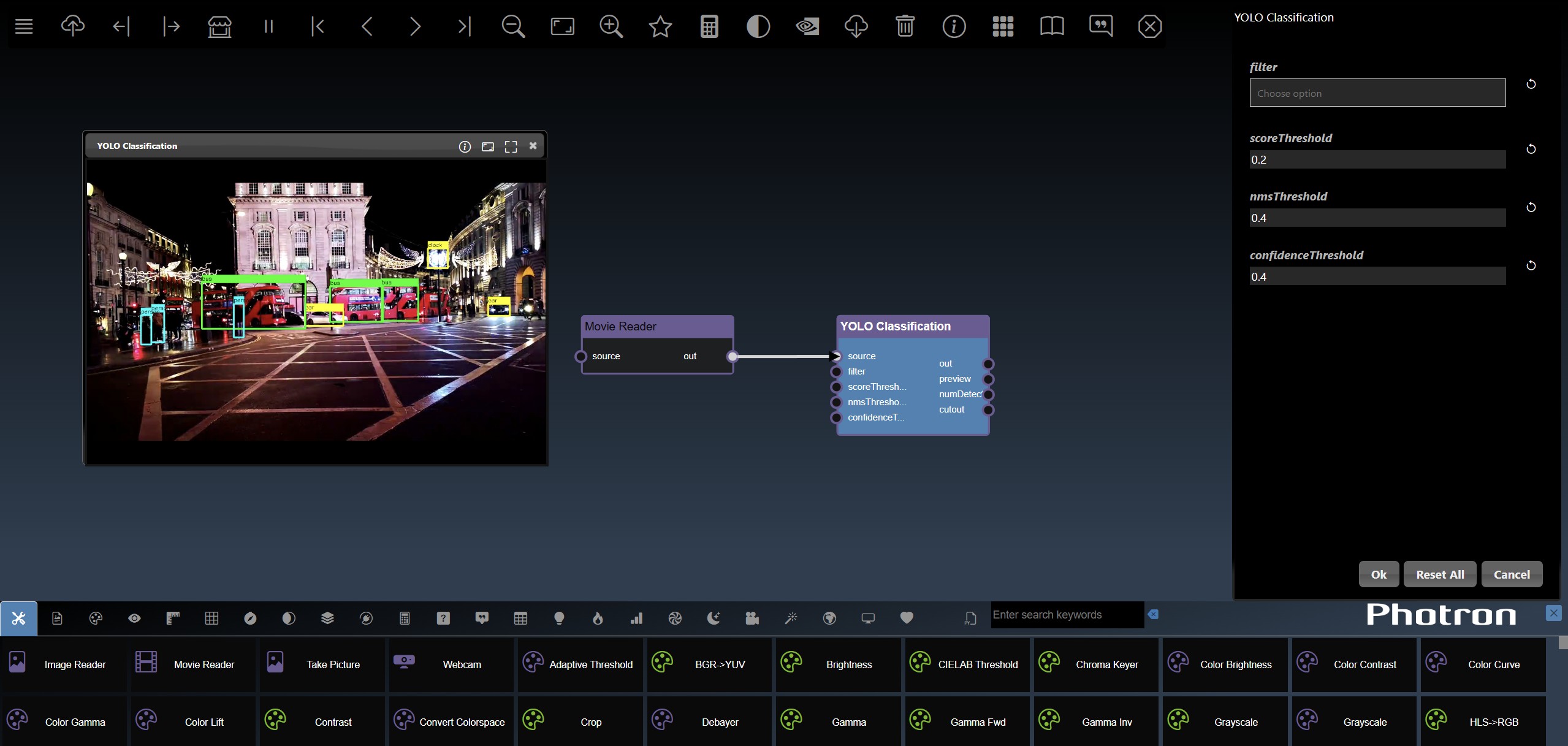
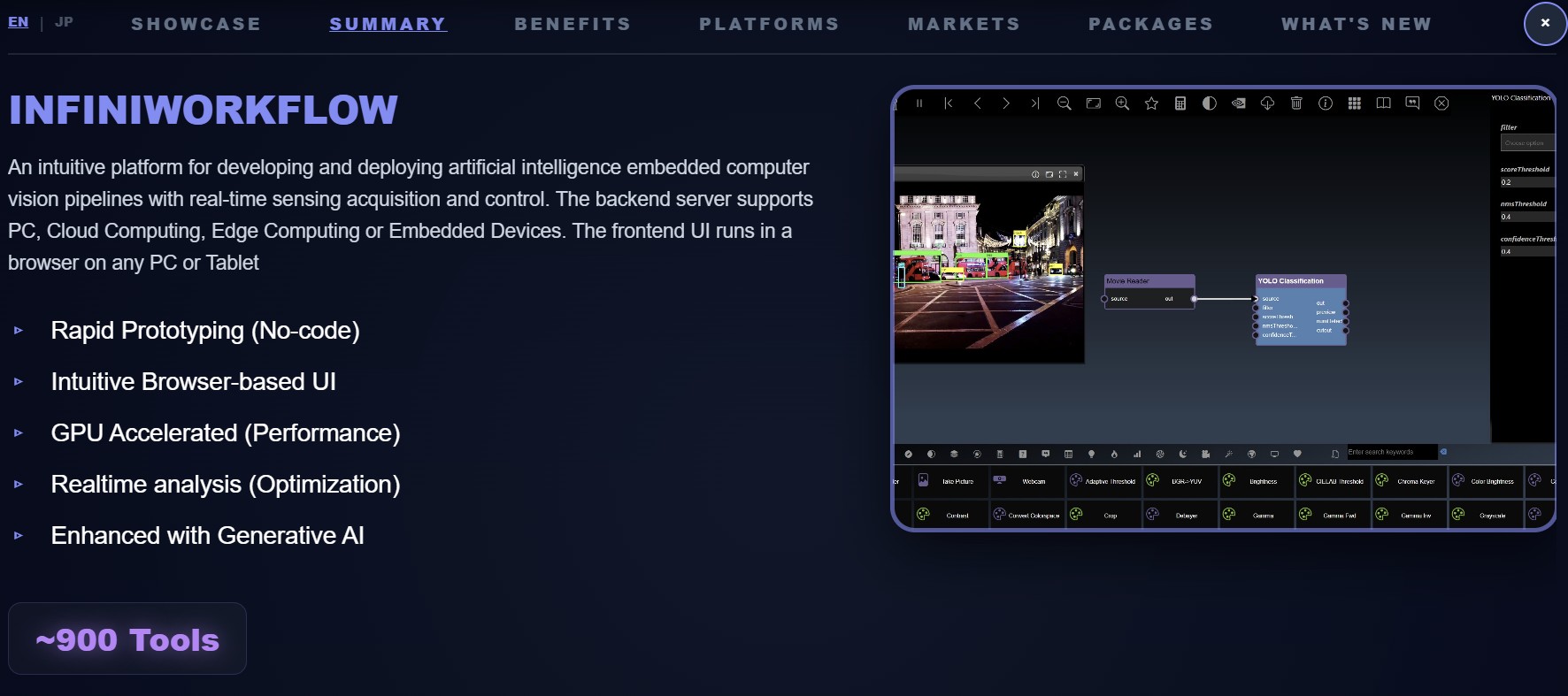
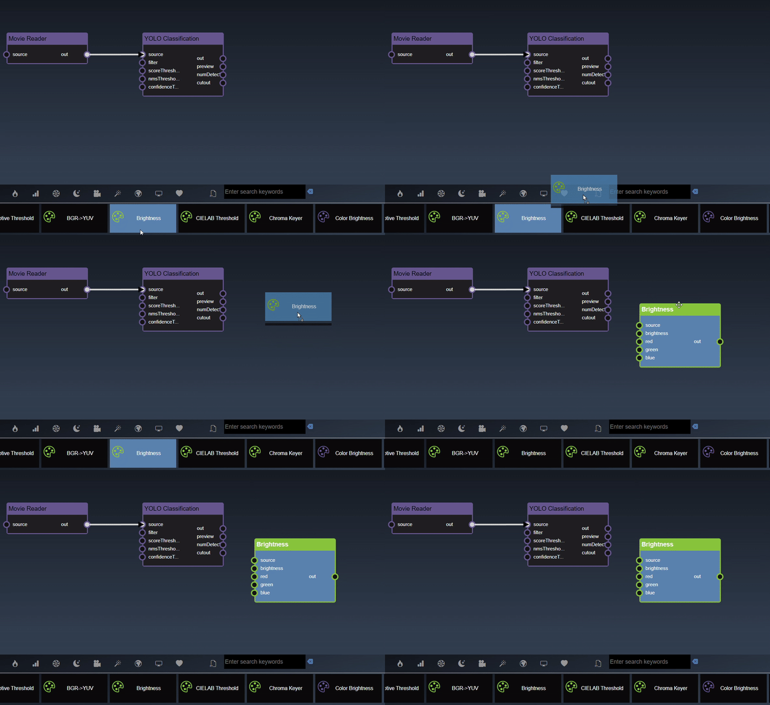
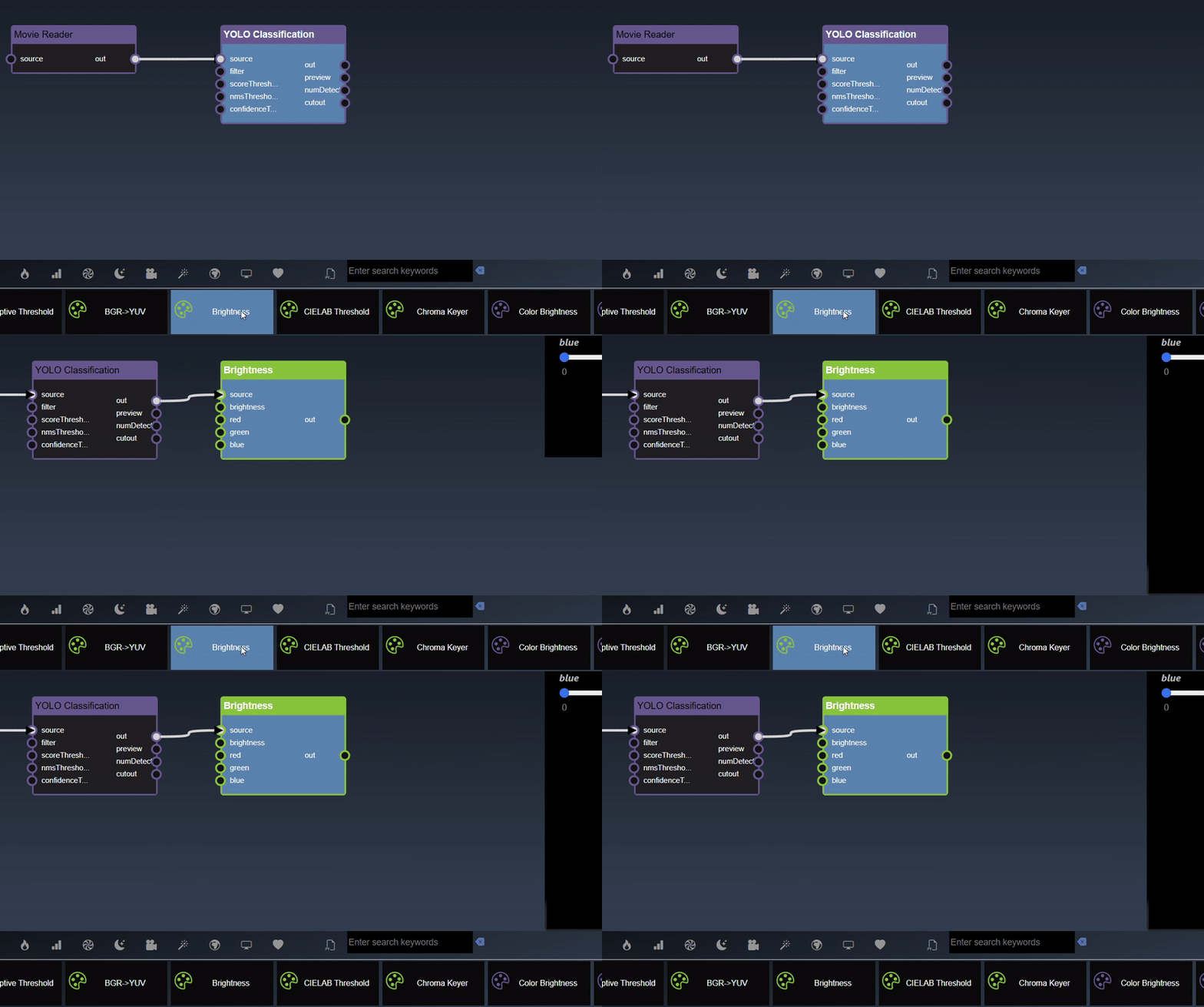
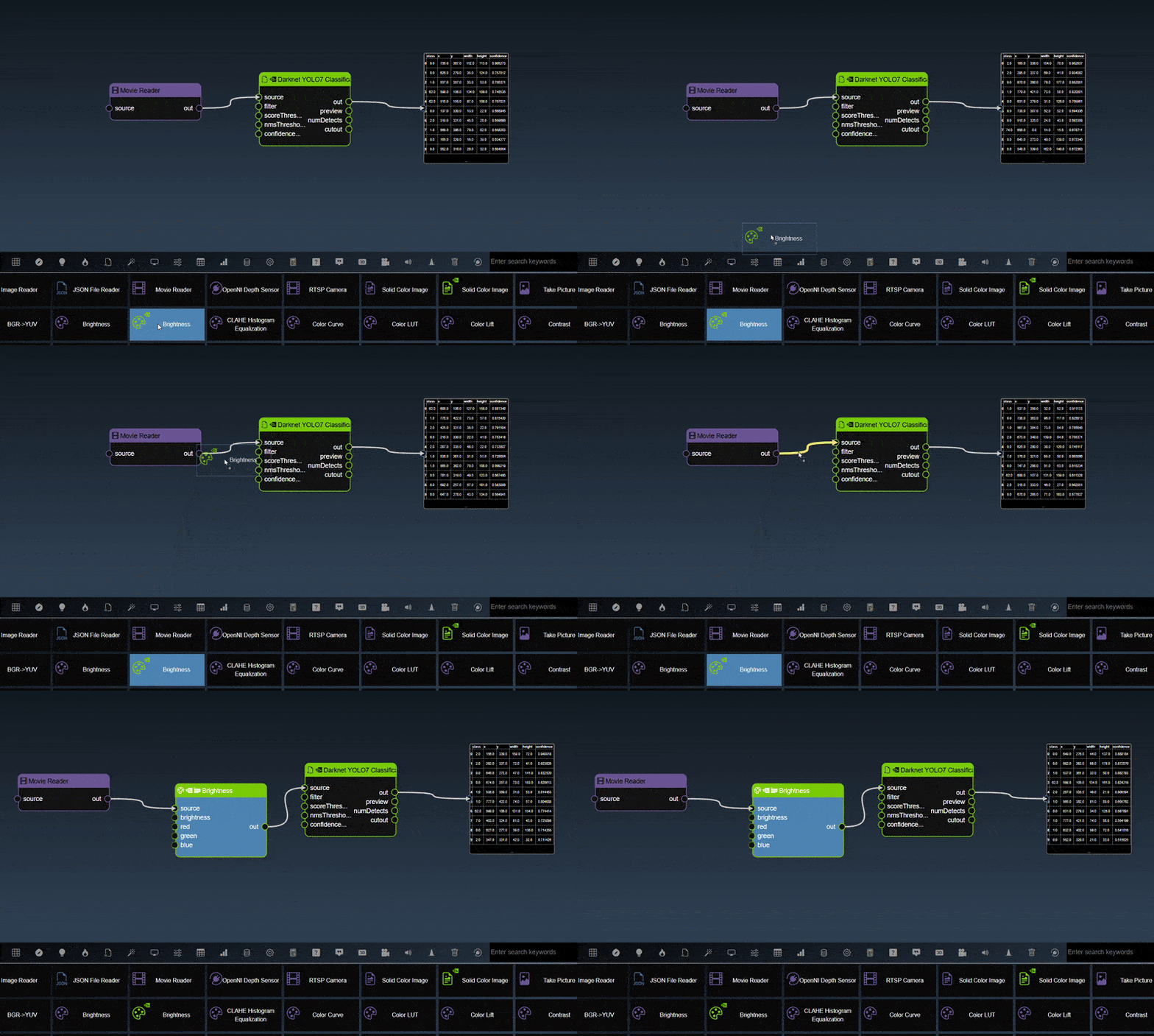

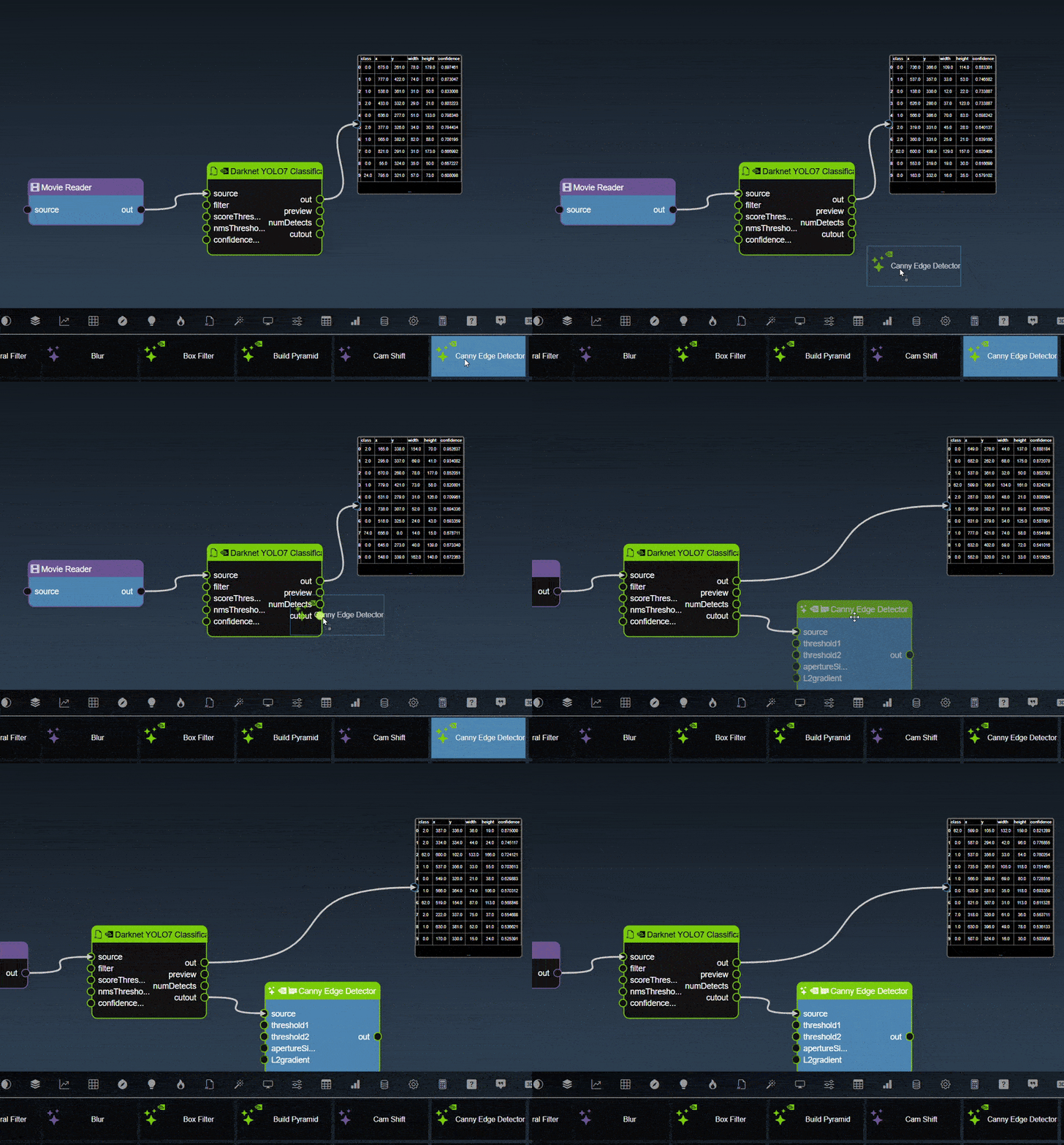
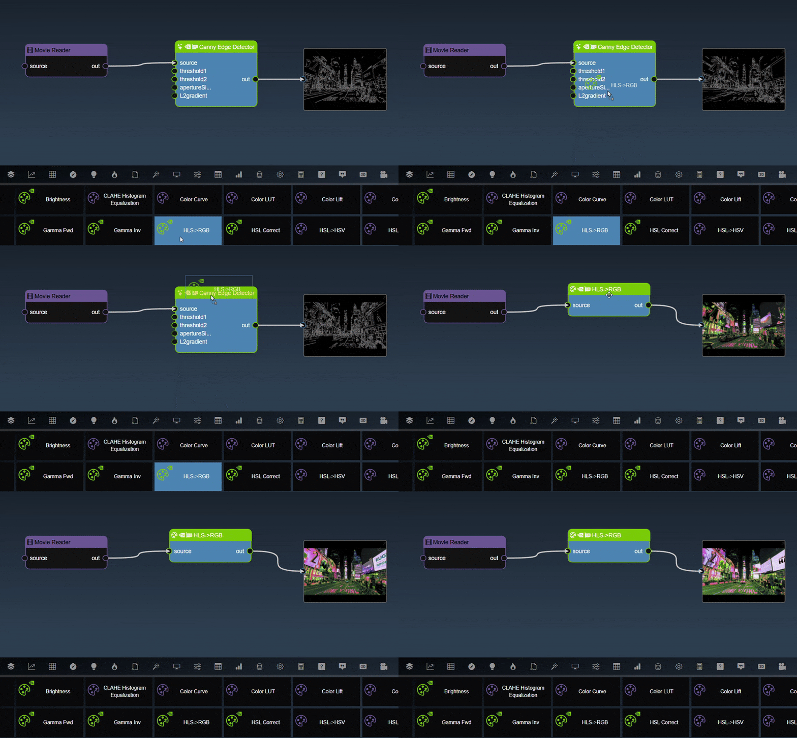
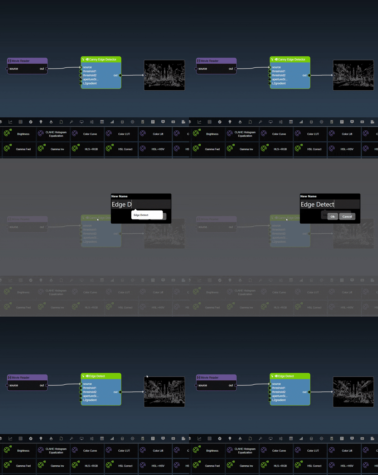
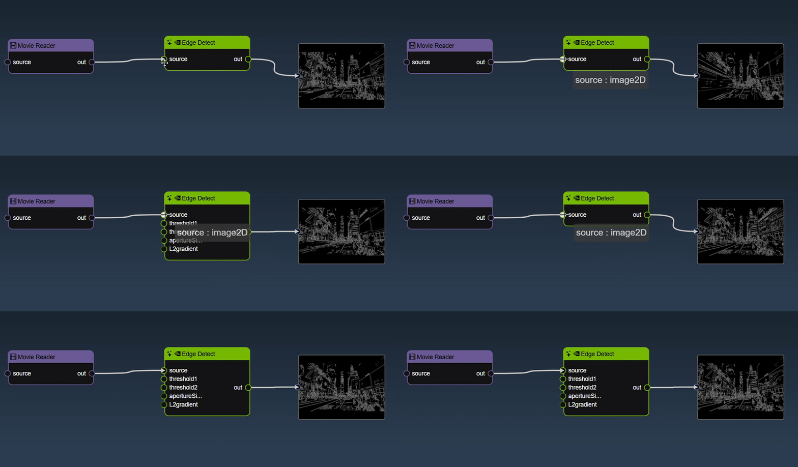


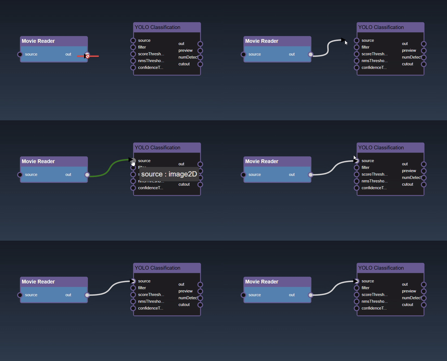
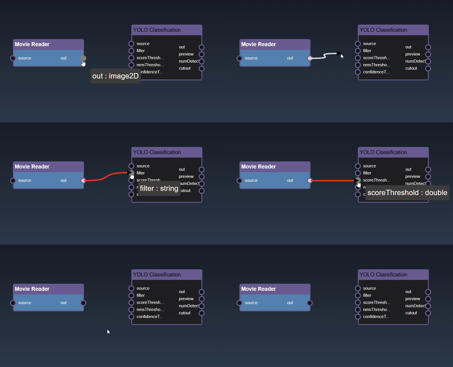
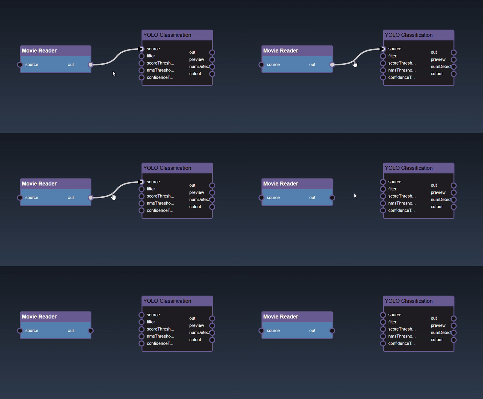
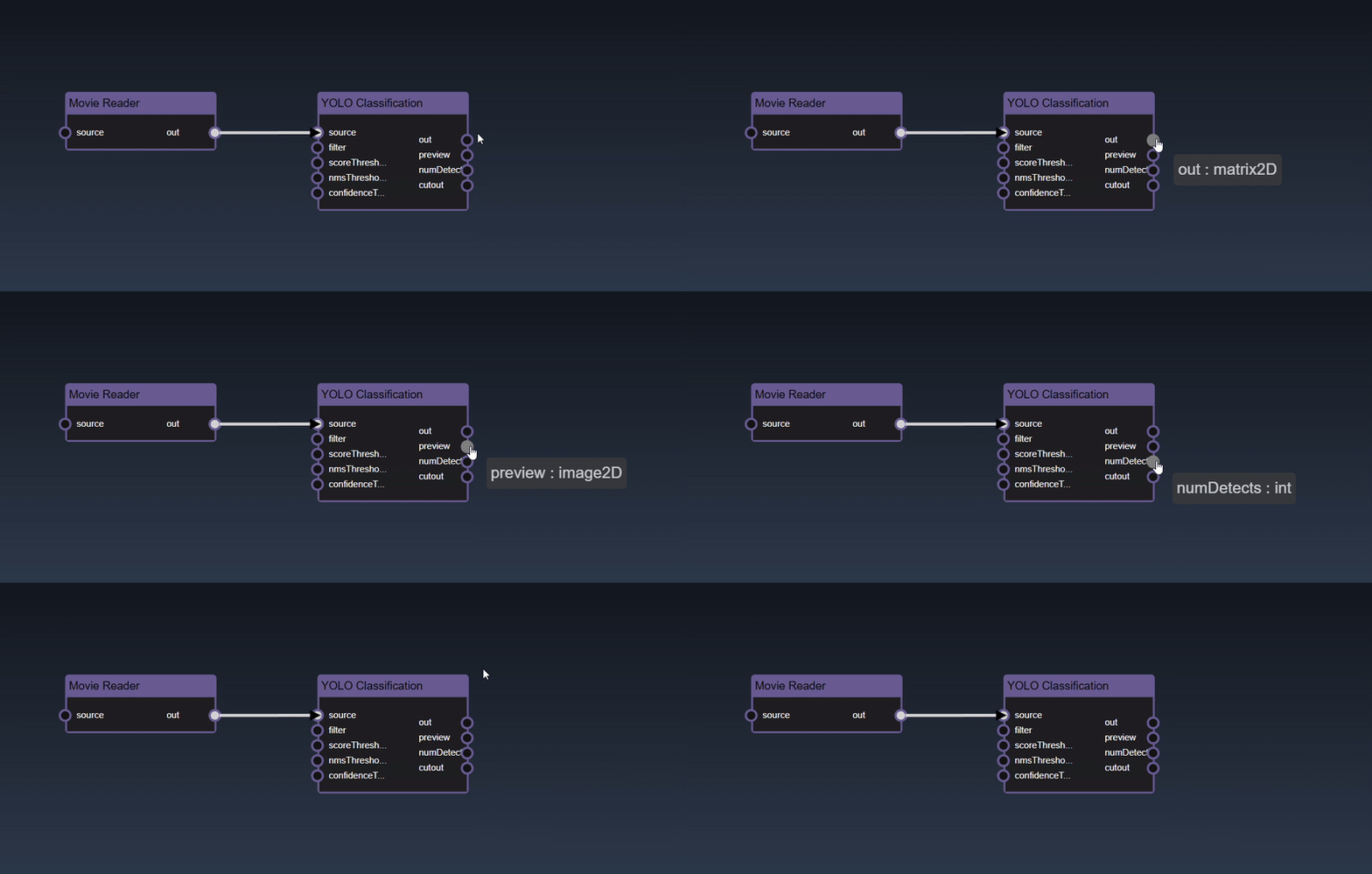
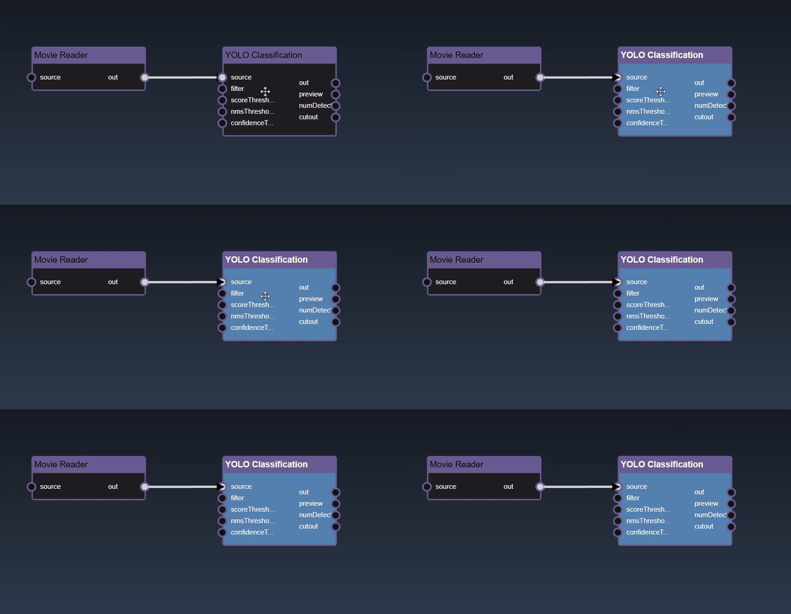
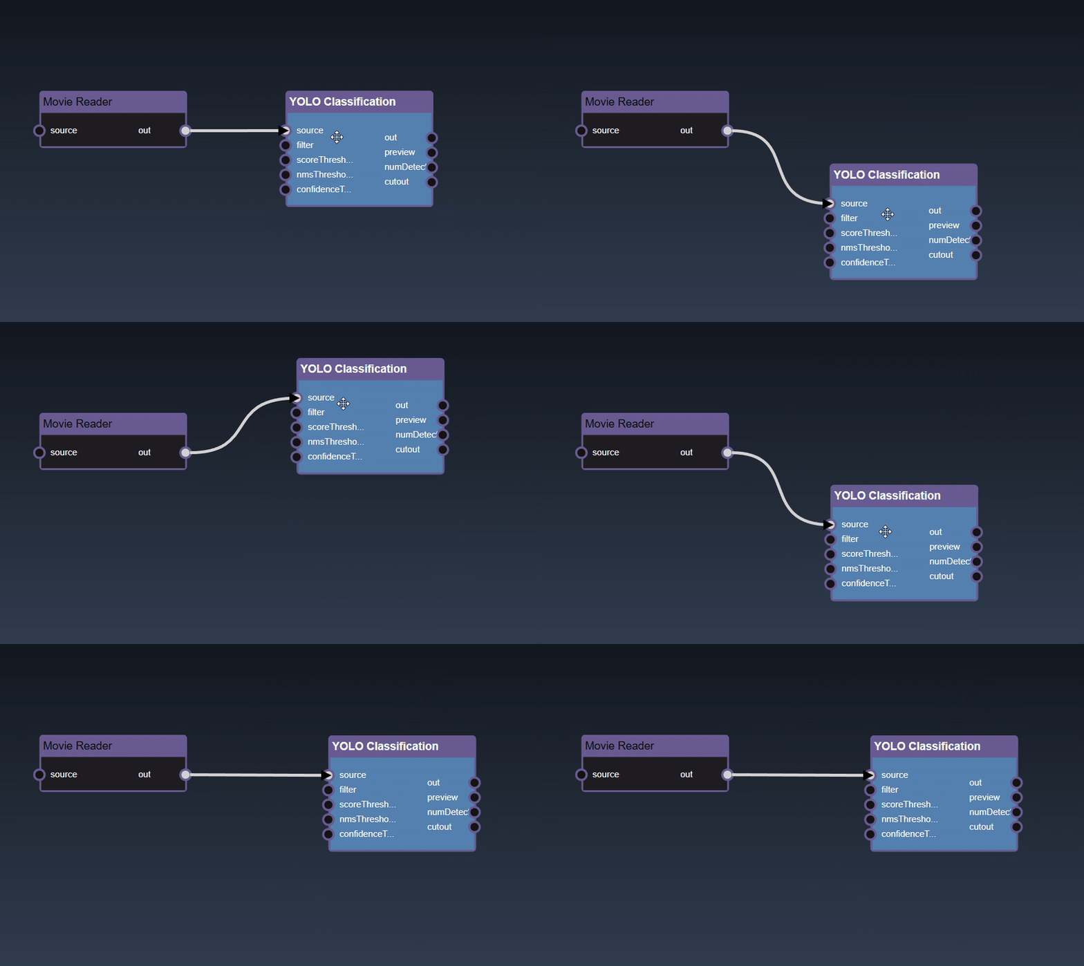
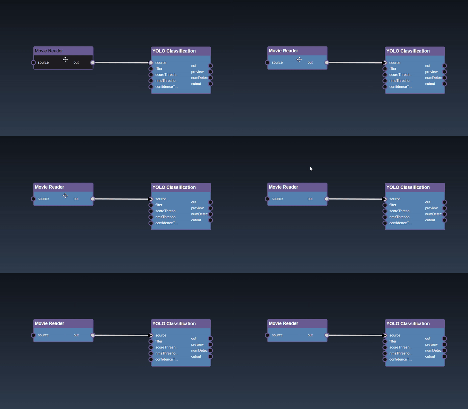
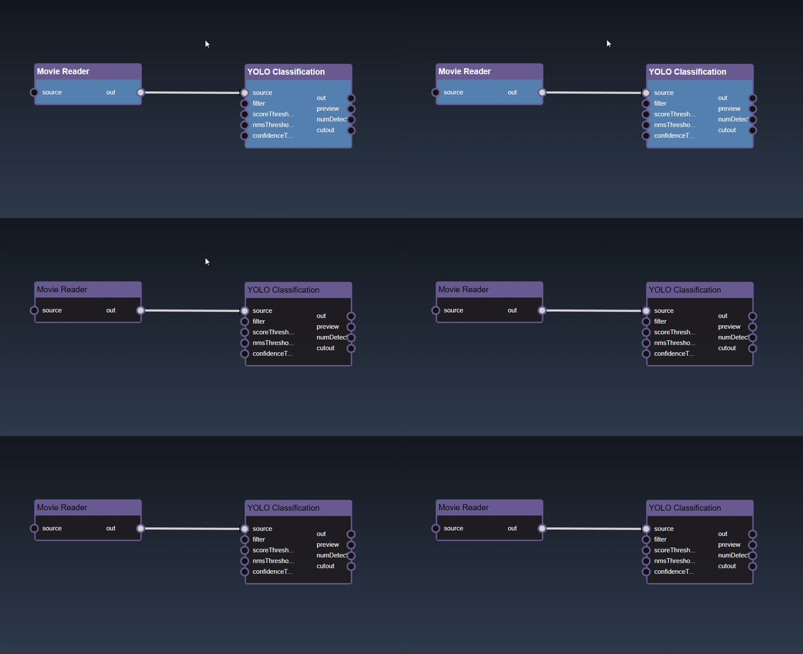
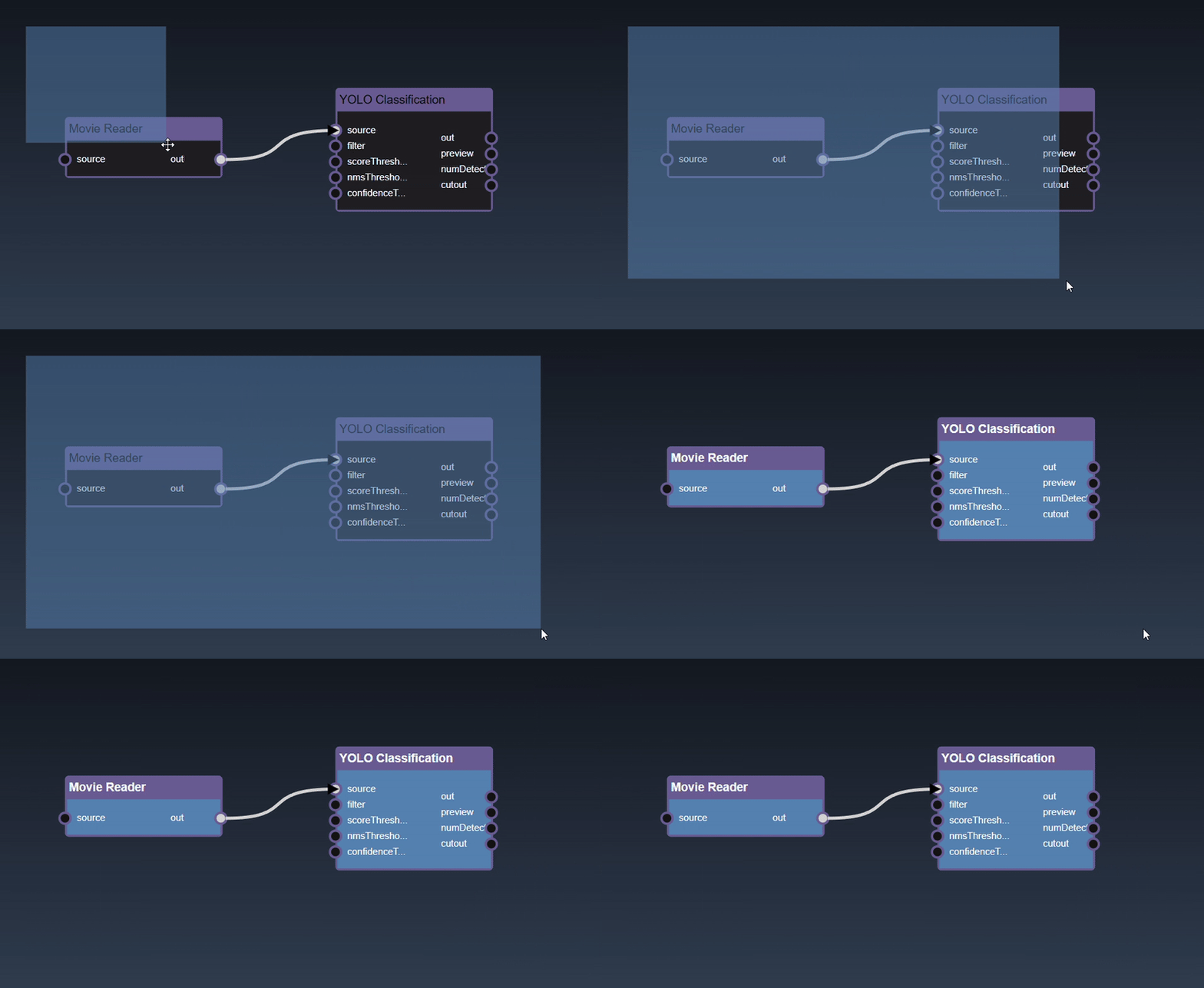
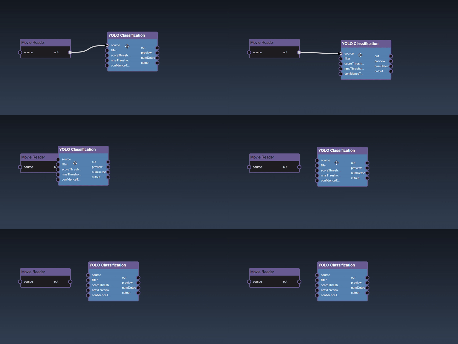

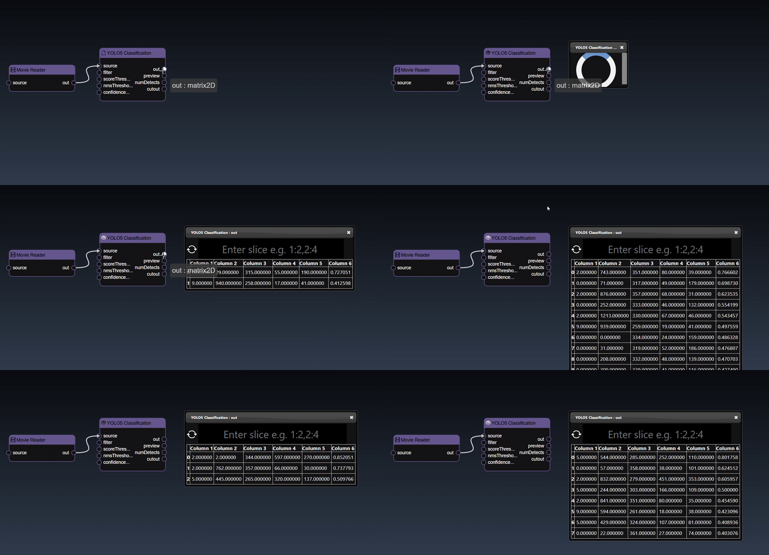
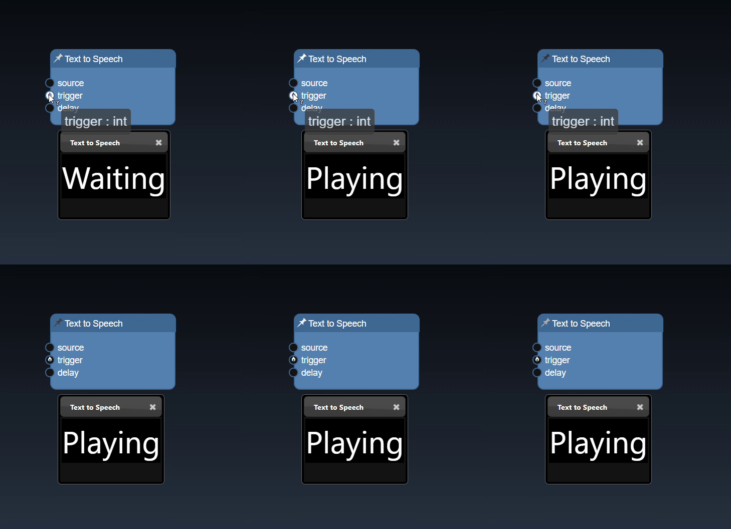

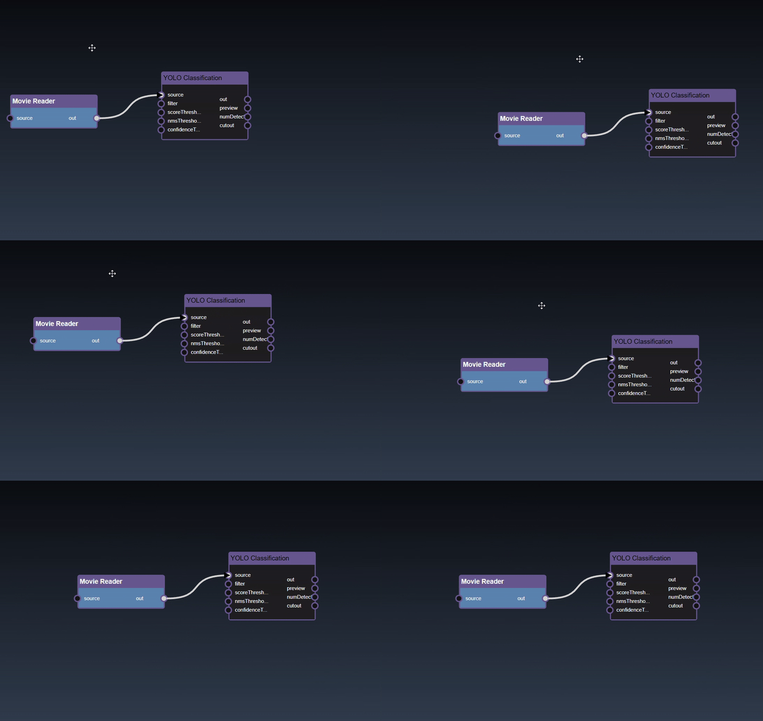
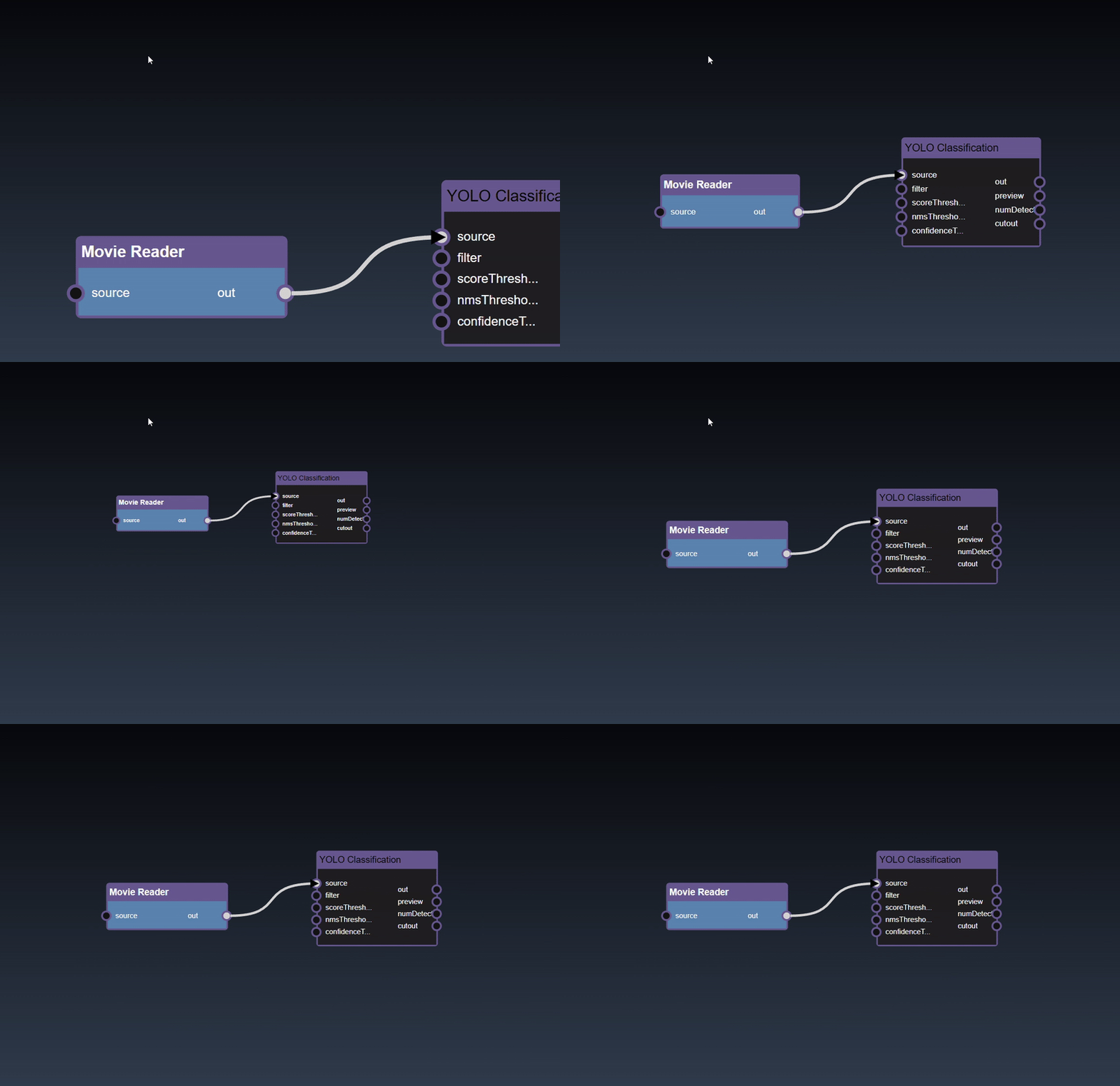
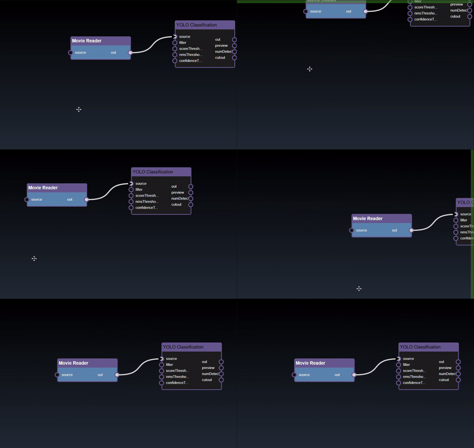
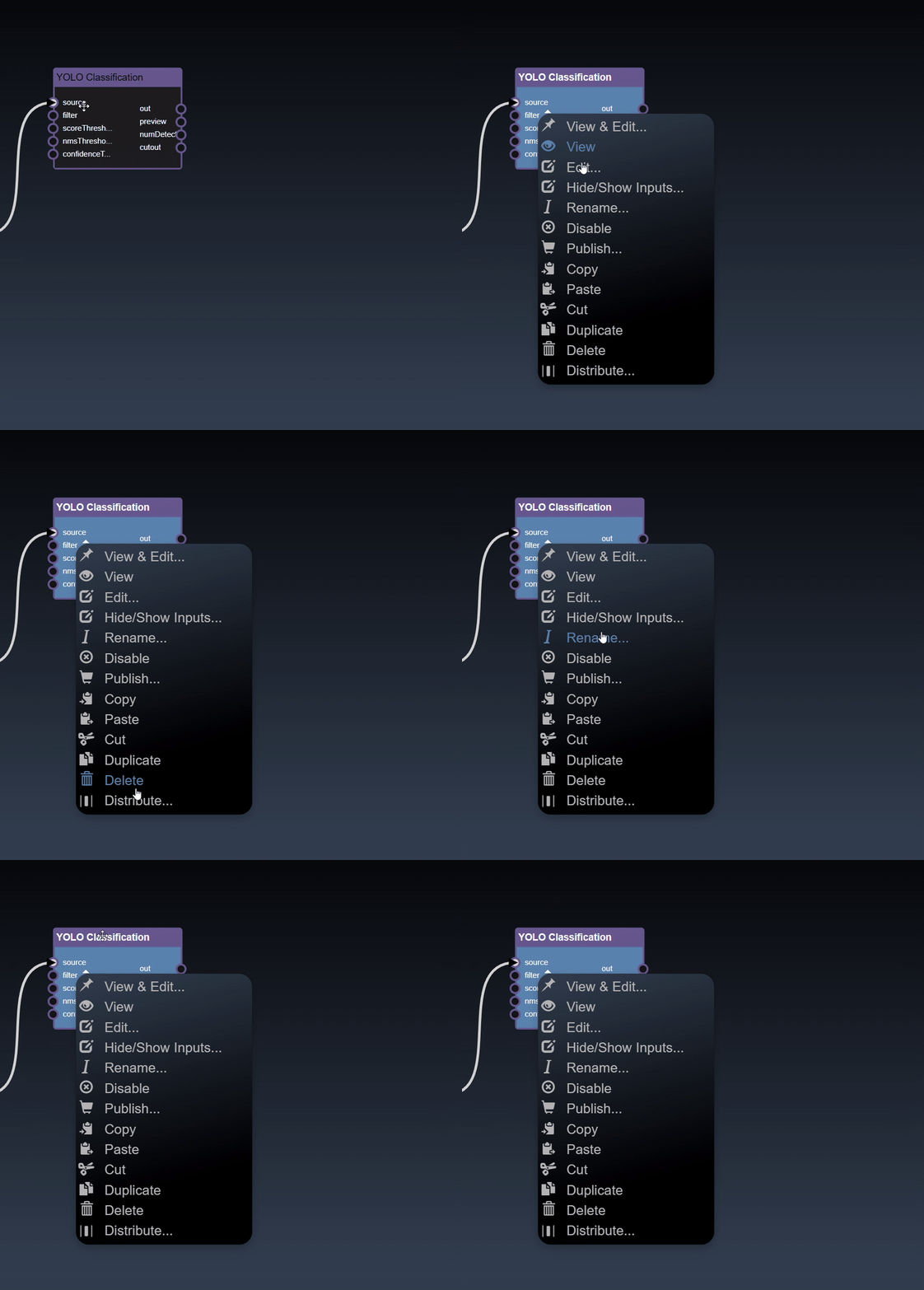
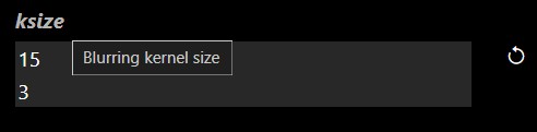

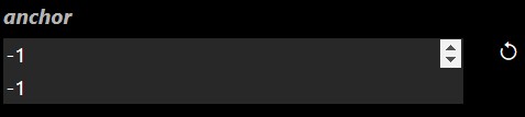

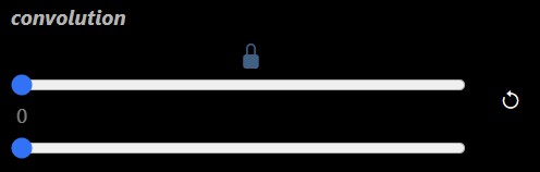


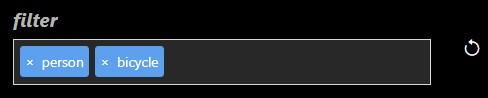
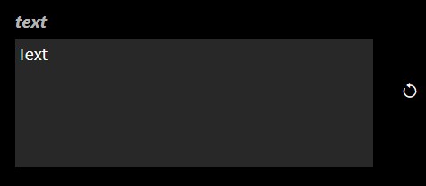


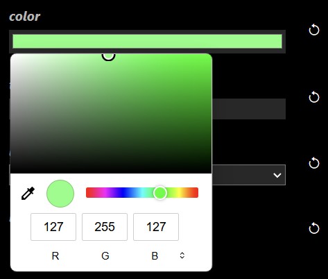

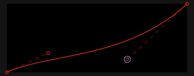
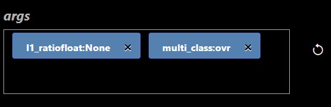
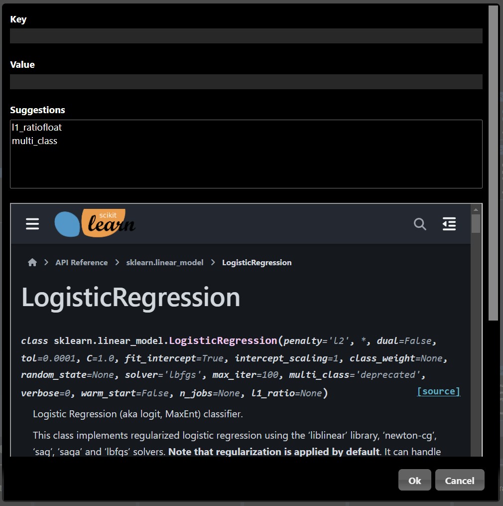

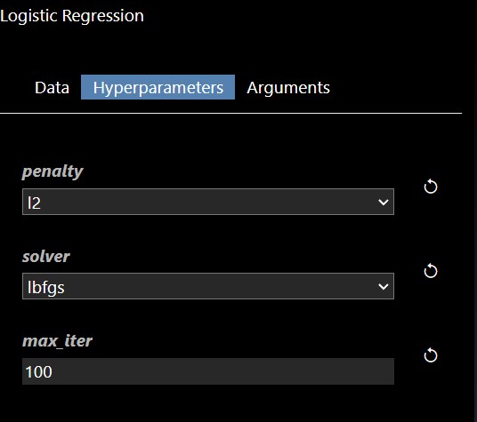
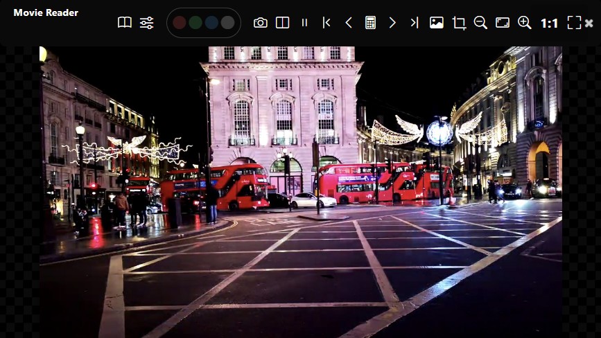
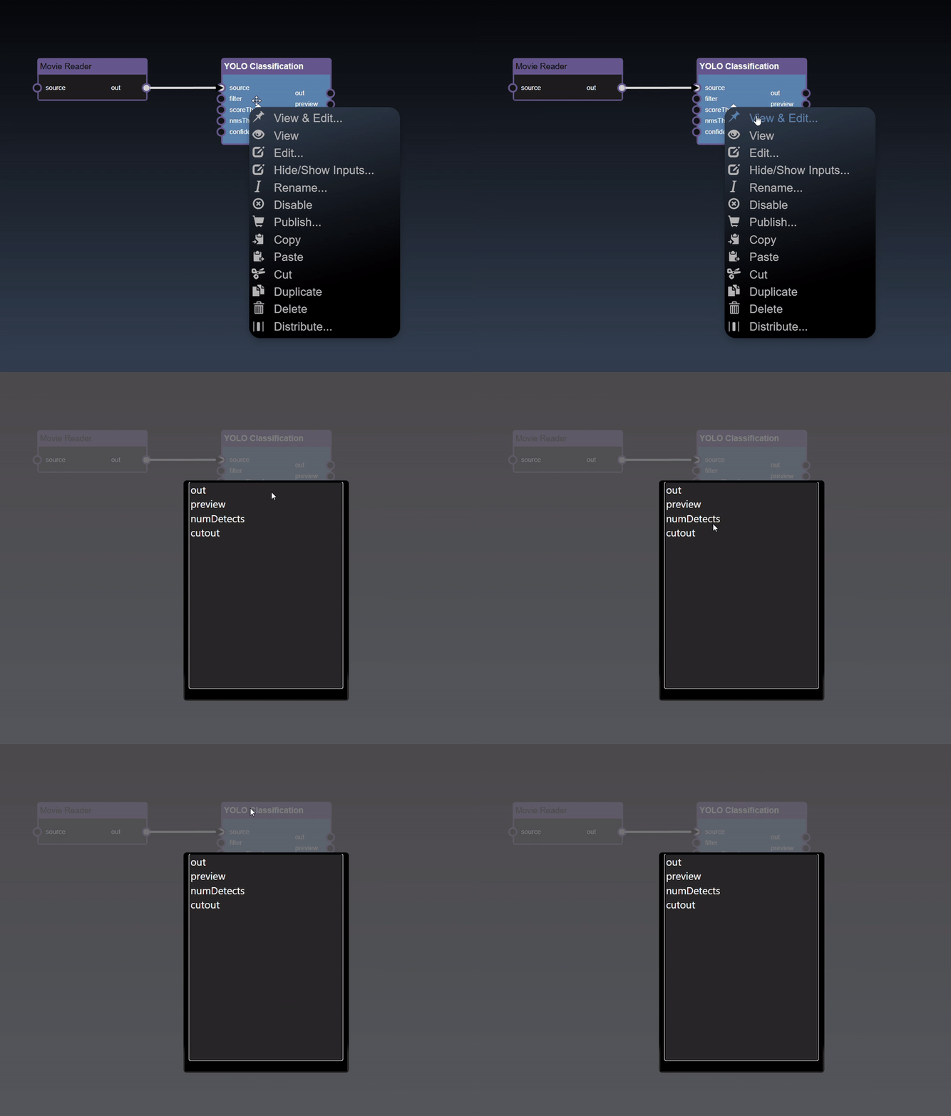
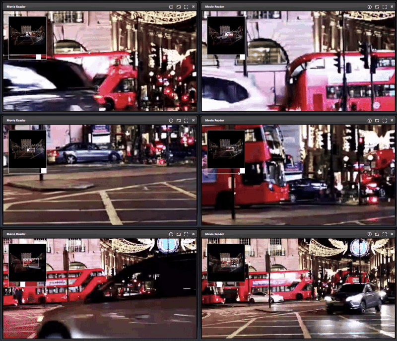
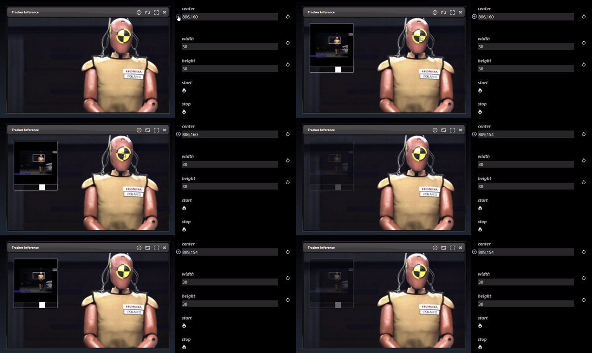
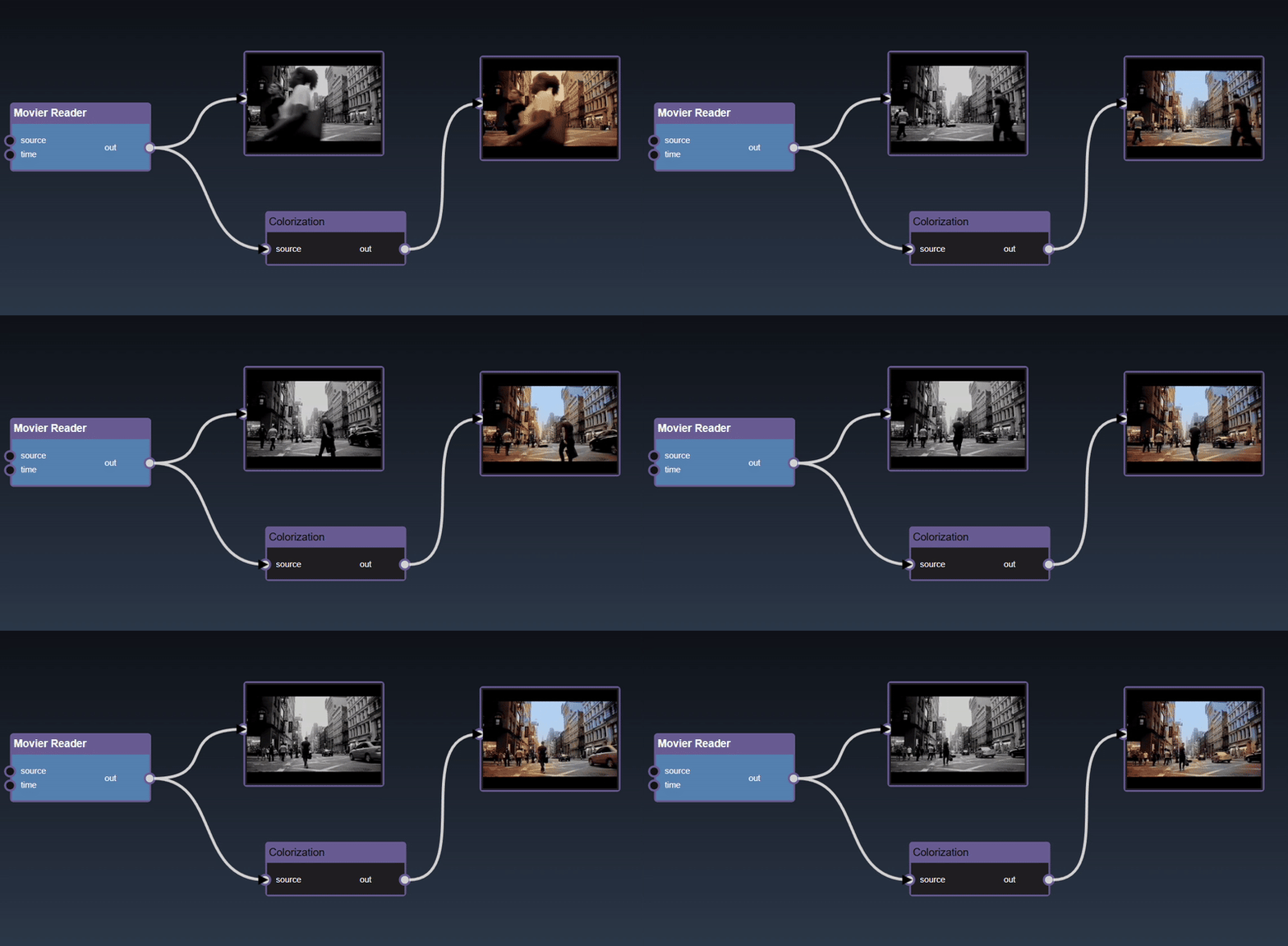


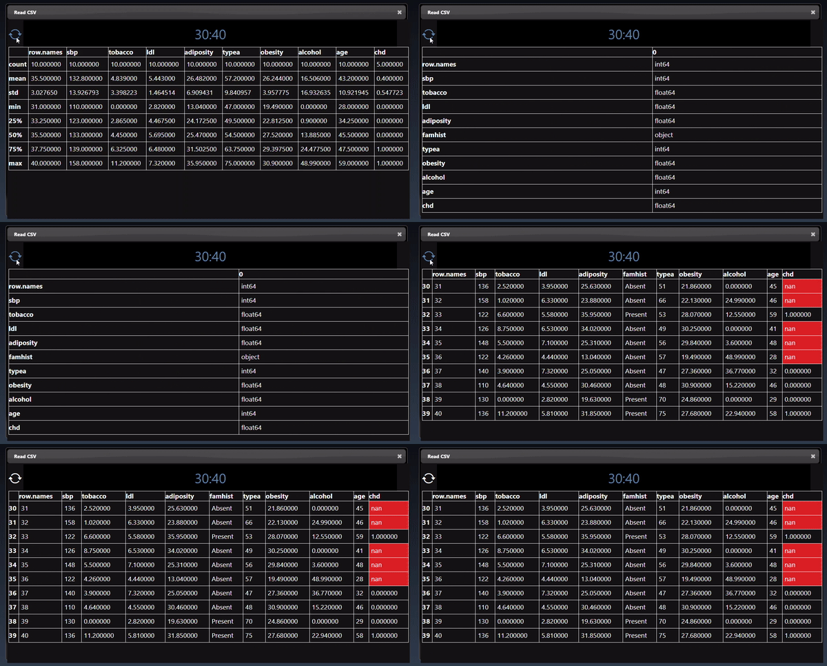
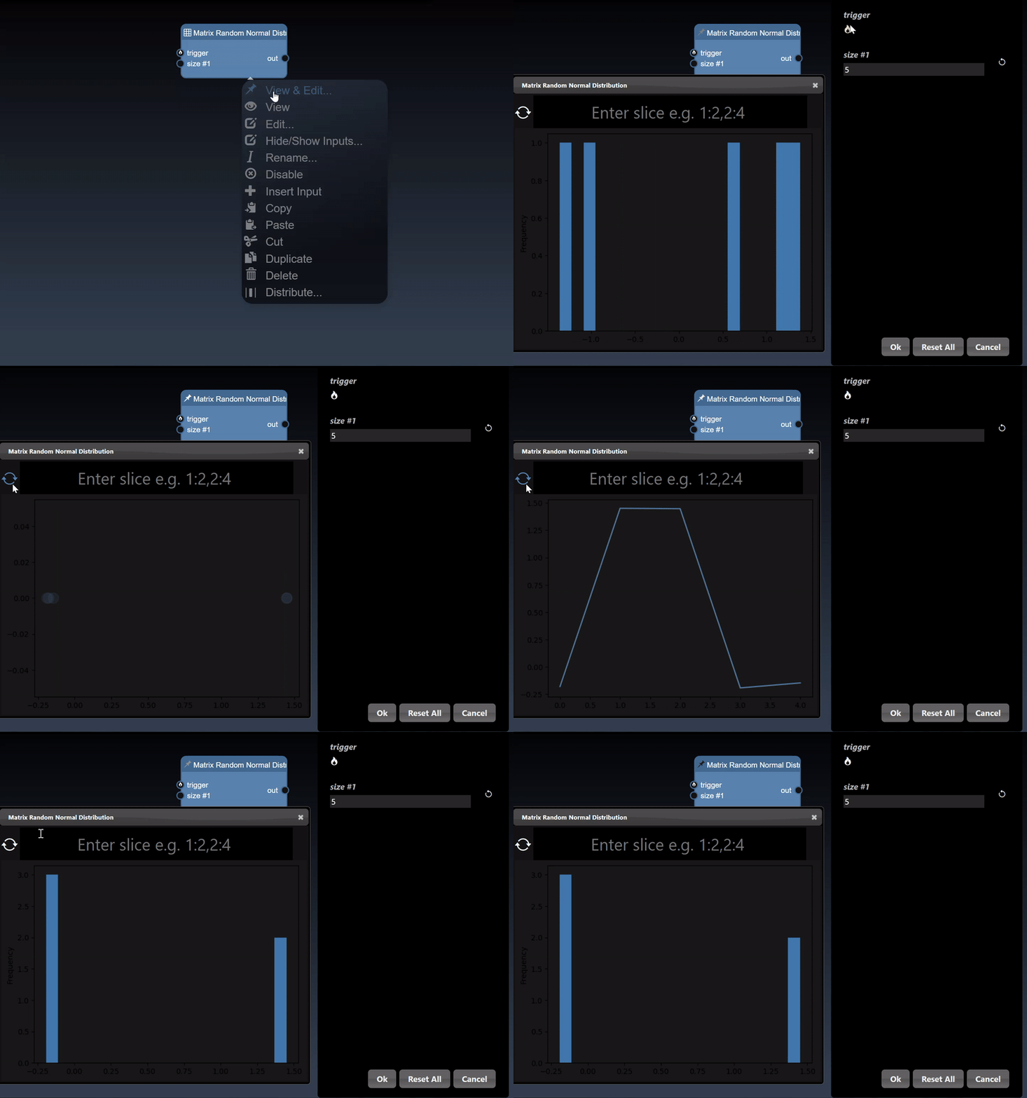
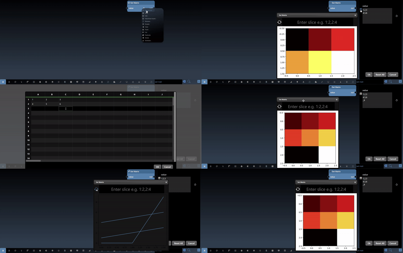
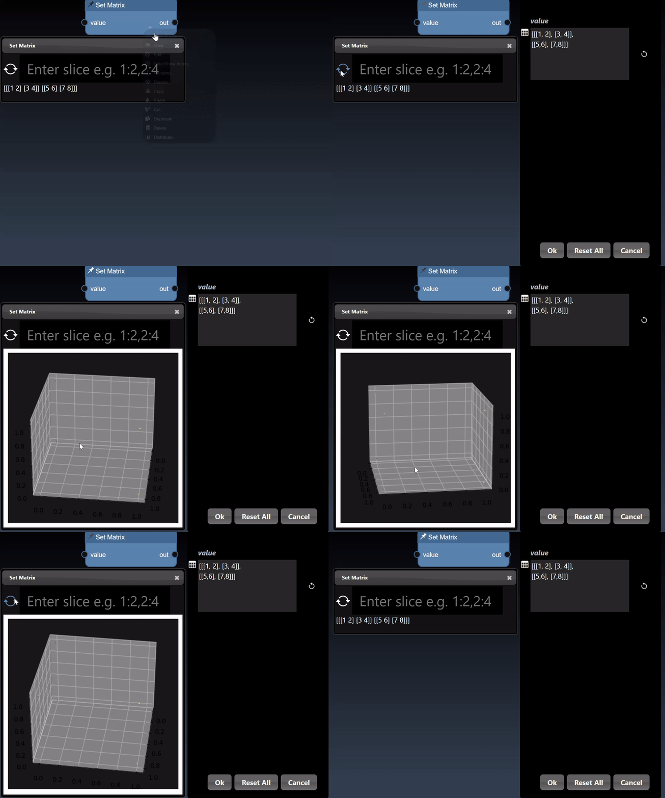
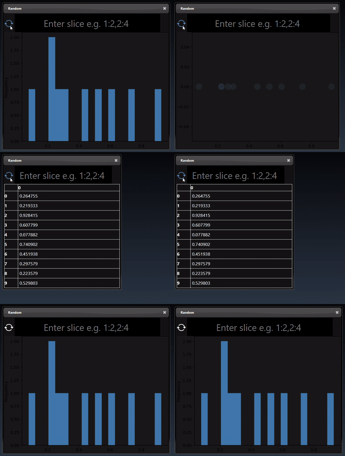
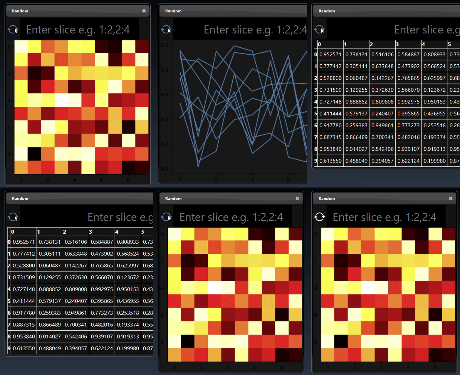
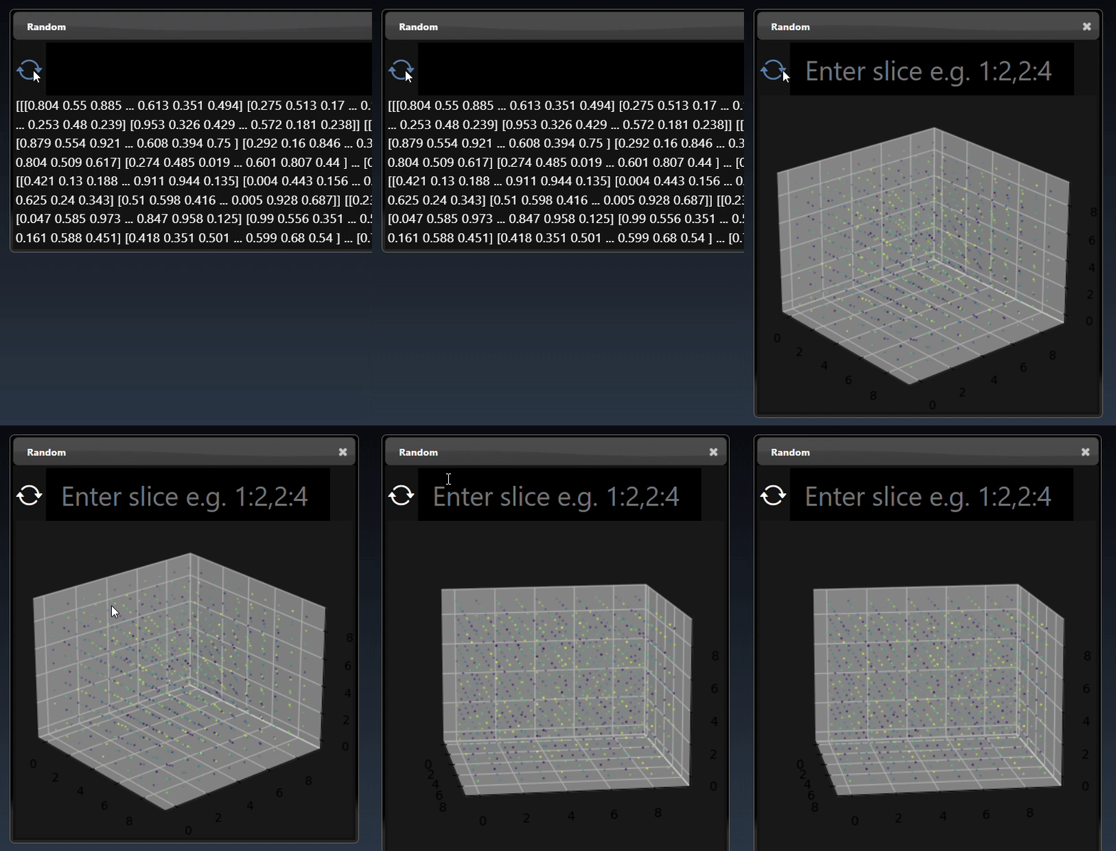
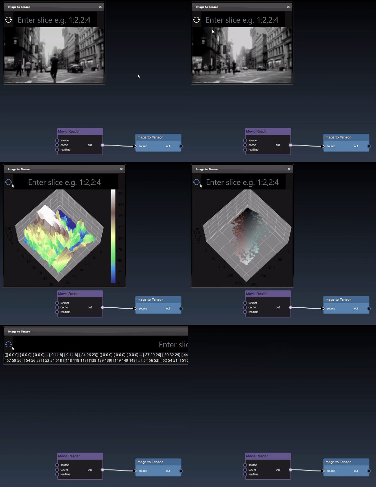
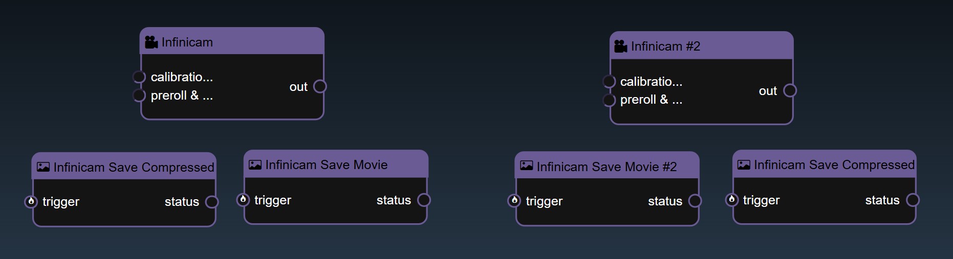


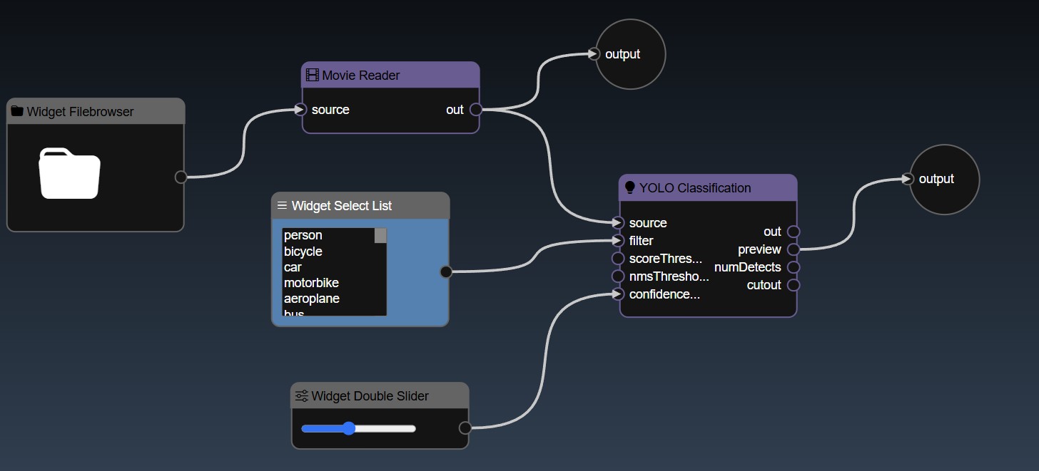
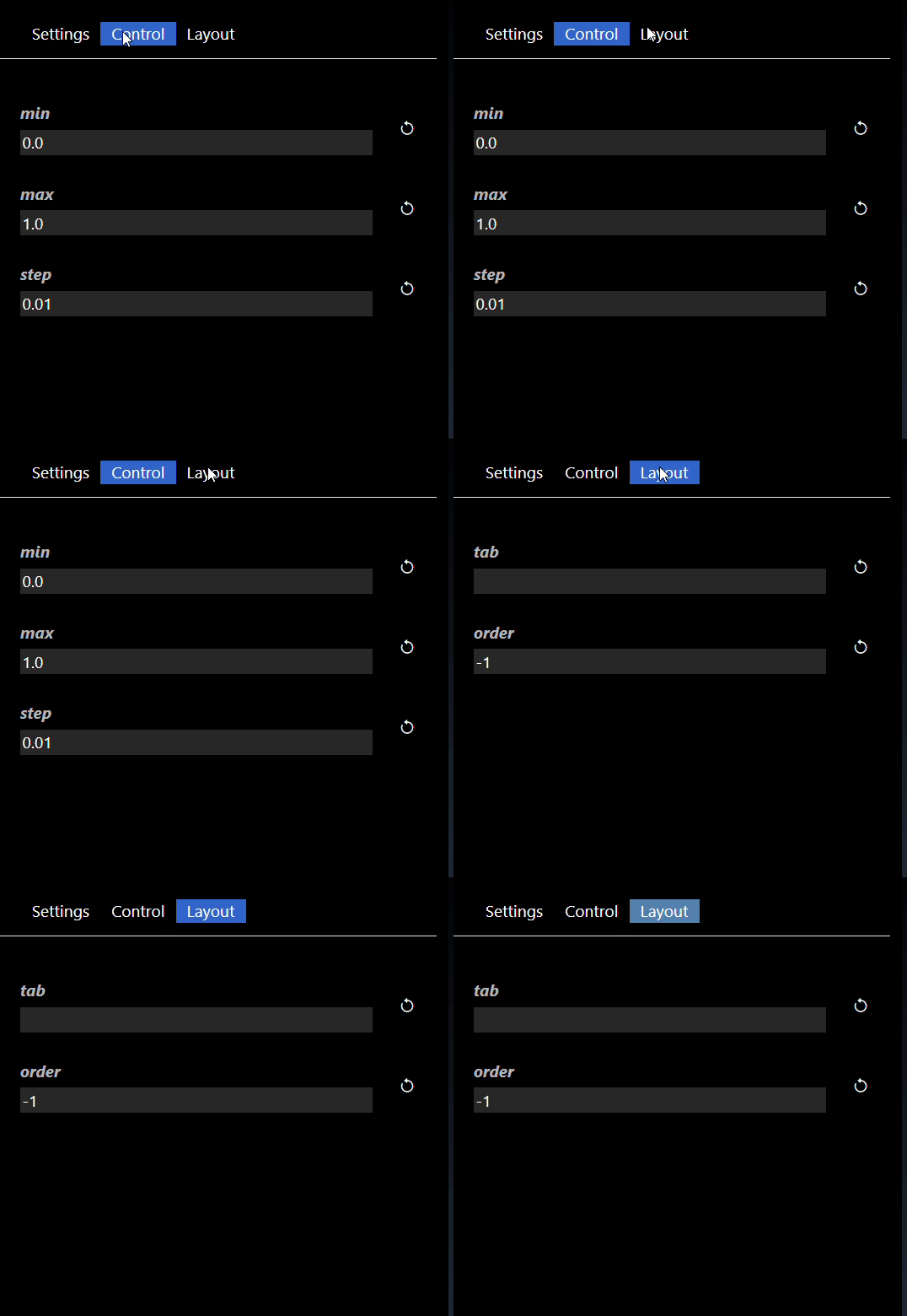
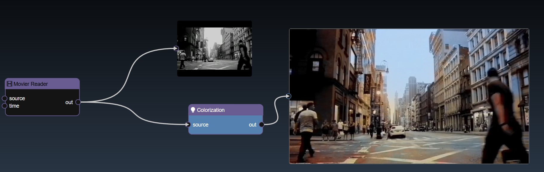
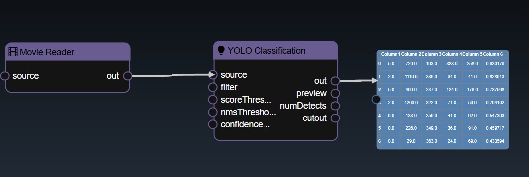
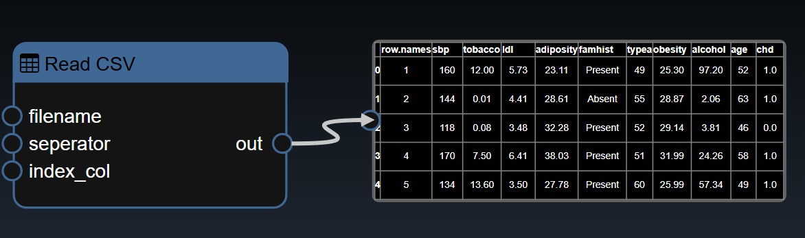
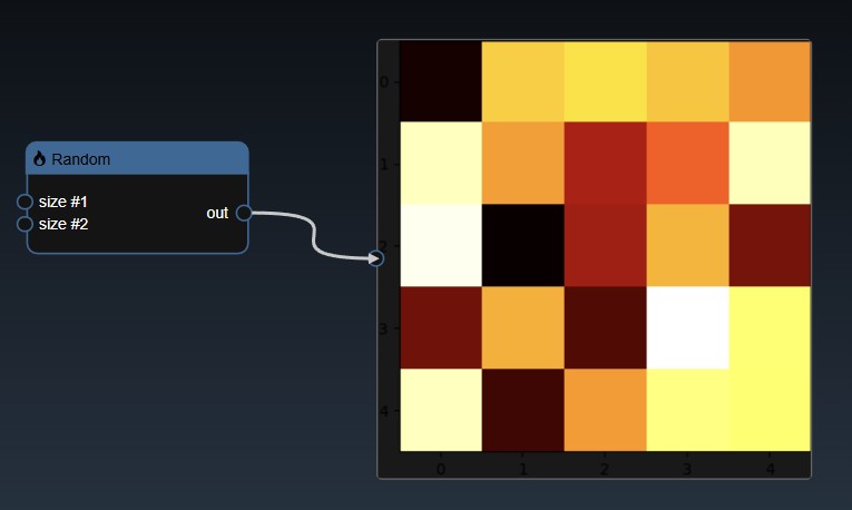
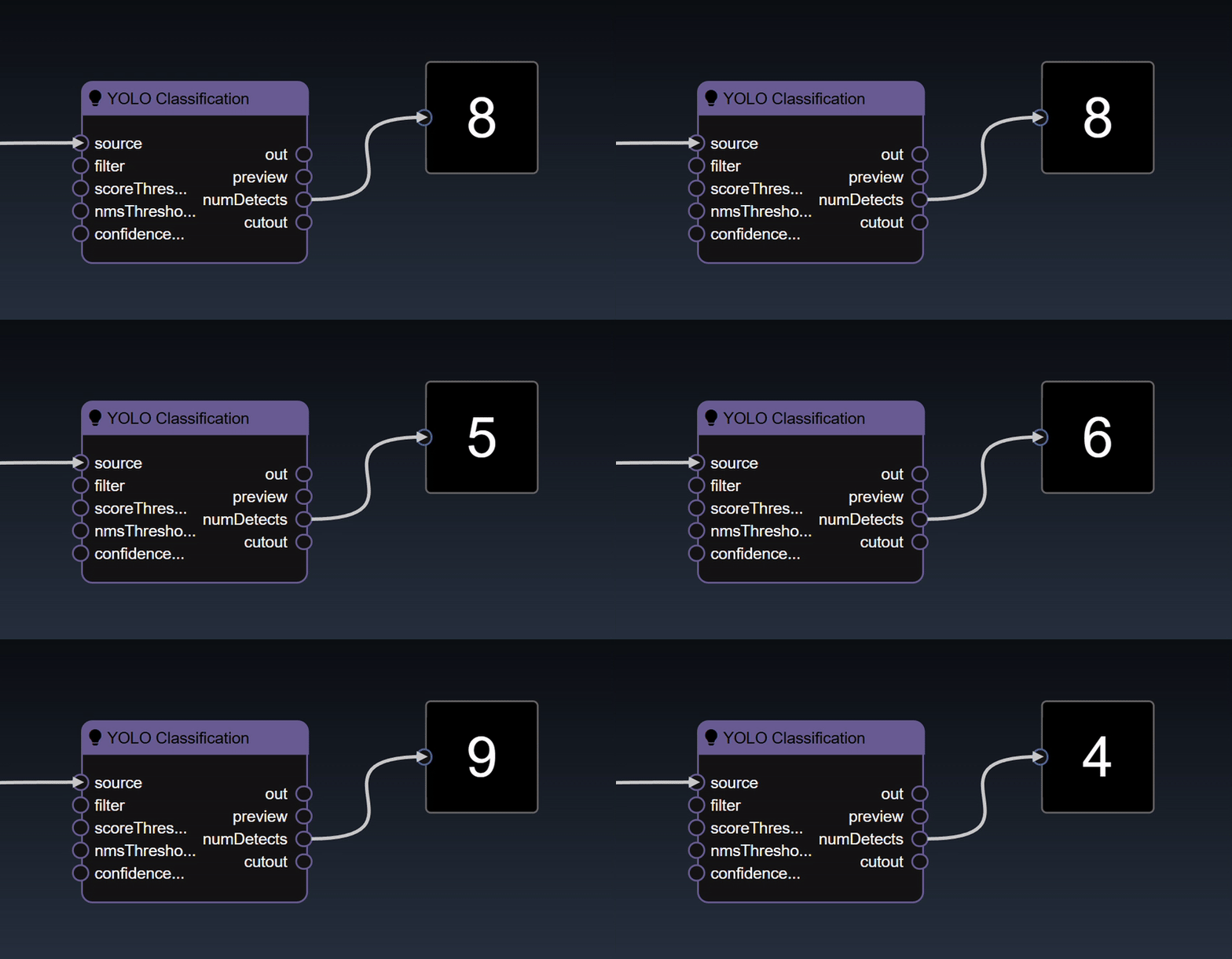
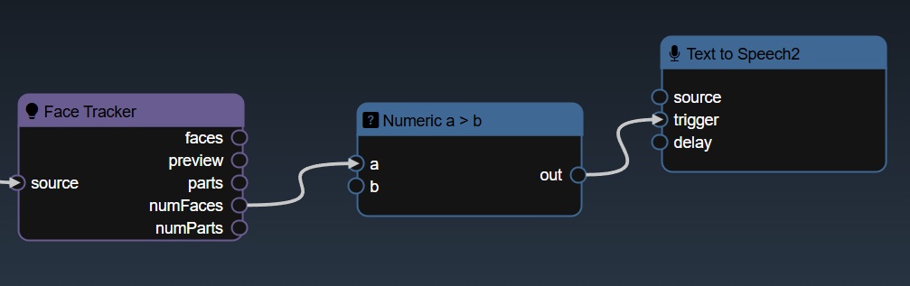
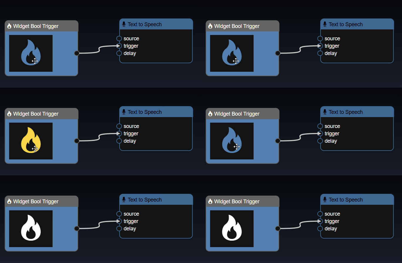
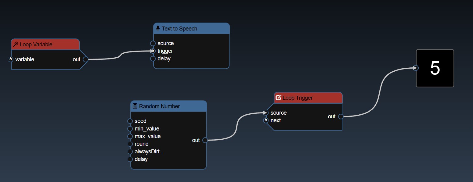
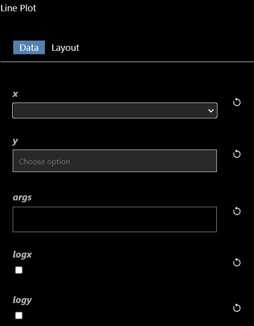
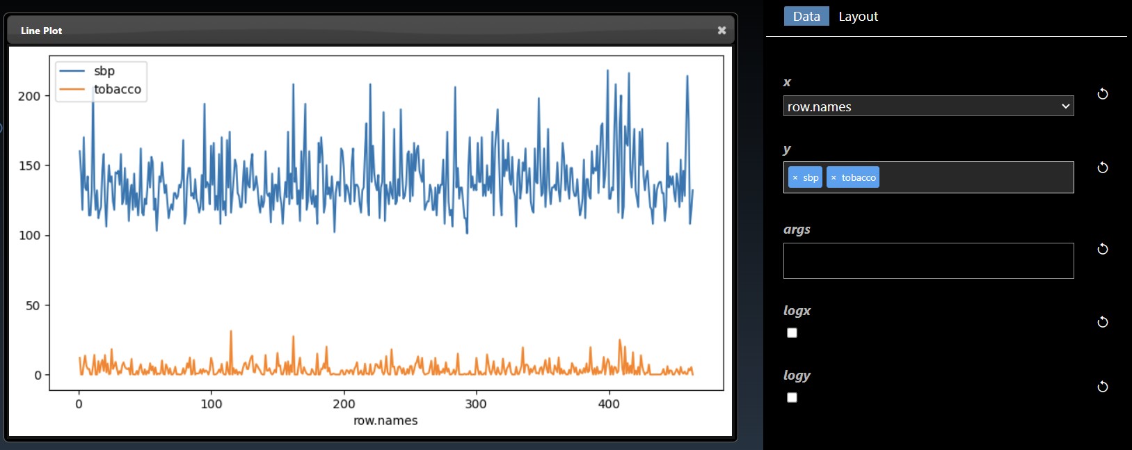
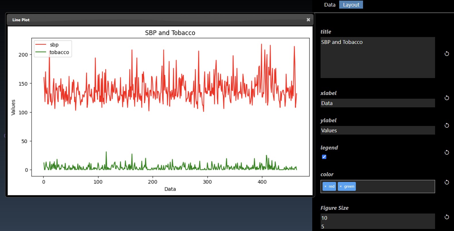
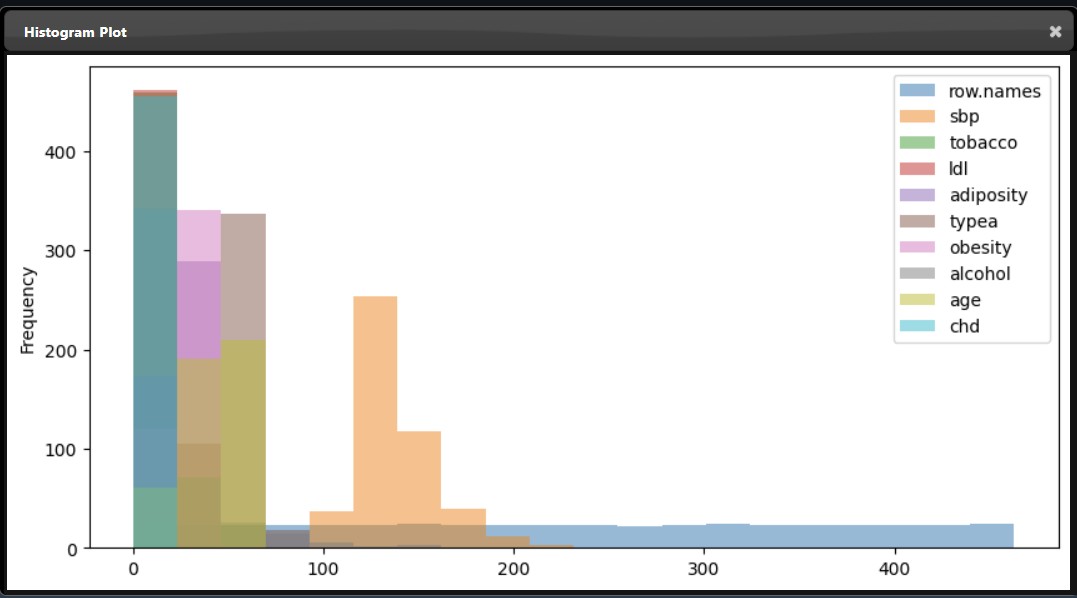
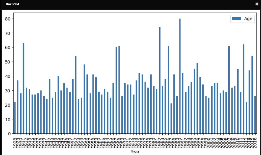
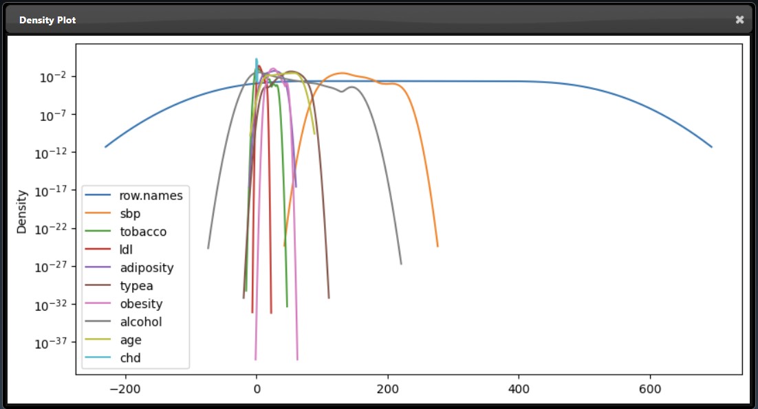
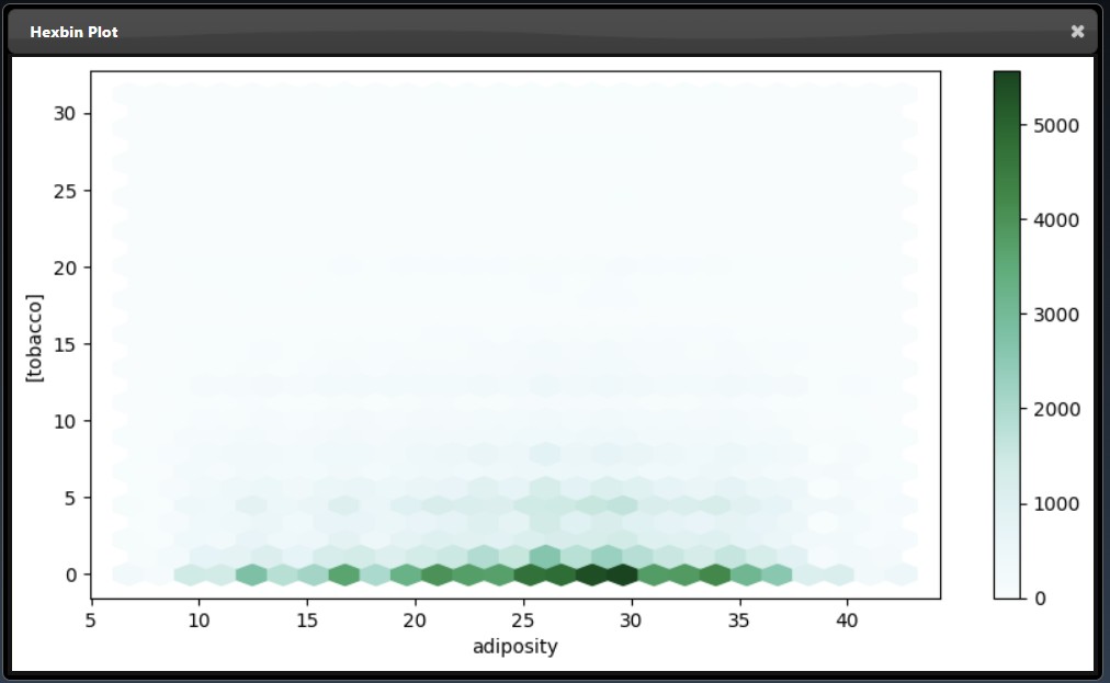
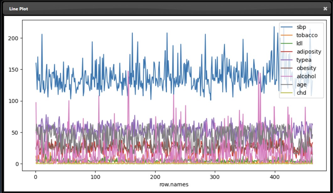
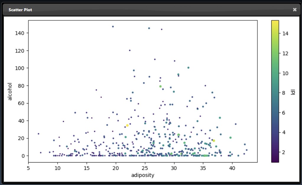
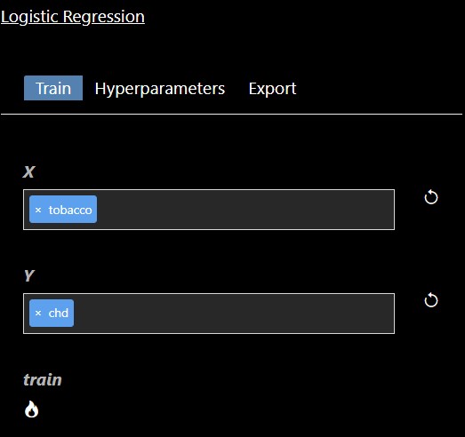
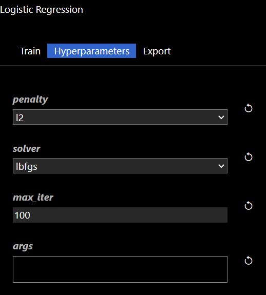
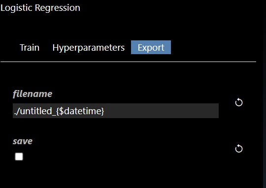
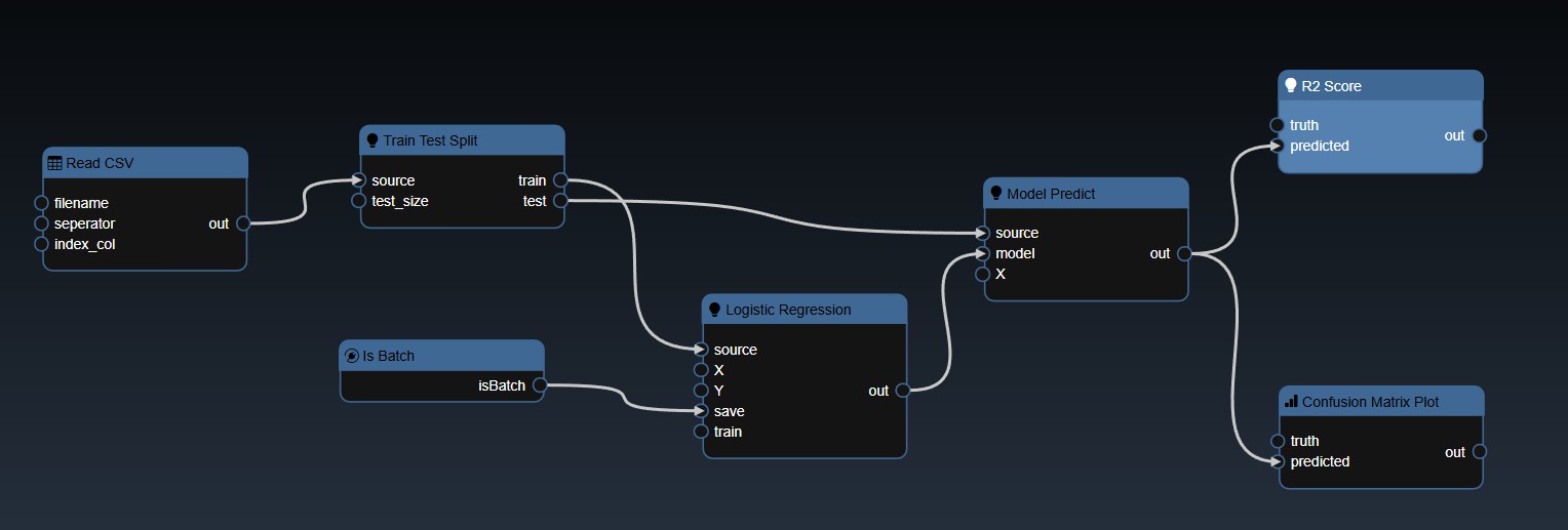
 Contours.json
 AI_Welding.json
 Color_Grade.json
 Live_Camera.json